Memory Management (a)
Explore the essential techniques and processes involved in managing memory for user programs, such as relocation, protection, sharing, overlays, and dynamic loading. Understand the role of Memory-Management Unit (MMU) and dynamic linking. Discover memory management schemes like paging, segmentation, and swapping for optimal utilization of memory resources.


Memory Management (a)
E N D
Presentation Transcript
Background • Program must be brought into memory and placed within a process for it to be run. • Input queue– collection of processes on the disk that are waiting to be brought into memory to run the program. • User programs go through several steps before being run.
Memory Management Requirements • Relocation • Users generally don’t know where they will be placed in main memory • May want to swap in at a different place (pointers???) • Generally handled by hardware • Protection • Prevent processes from interfering with the O.S. or other processes • Often integrated with relocation • Sharing • Allow processes to share data/programs • Logical Organization • Support modules, shared subroutines • Physical Organization • Main memory verses secondary memory • Overlaying
von Neumann Model • Instruction cycle • CPU fetches instructions from memory • Instruction is decoded • Operands loaded from memory • Instruction is executed • Results are then stored back in memory • Memory only sees a stream of addresses • requests • stores • “von Neumann Bottleneck”
Address Binding • A process must be tied to a physical address at some point (bound) • Binding can take place at 3 times • Compile time • Always loaded to same memory address • must recompile code if starting location changes • Load time • relocatable code • stays in same spot once loaded • Execution time • Binding delayed until run time • may be moved during execution • special hardware needed
Logical vs. Physical Address Space • The concept of a logical address space that is bound to a separate physicaladdress space is central to proper memory management. • Logical address– generated by the CPU; also referred to as virtual address. • Physical address– address seen by the memory unit. • Logical and physical addresses are the same in compile-time and load-time address-binding schemes; logical (virtual) and physical addresses differ in execution-time address-binding scheme.
Memory-Management Unit (MMU) • Hardware device that maps virtual to physical address. • In MMU scheme, the value in the relocation register is added to every address generated by a user process at the time it is sent to memory. • The user program deals with logical addresses; it never sees the real physical addresses.
Dynamic Loading • Routine is not loaded until it is called • Better memory-space utilization; unused routine is never loaded. • Useful when large amounts of code are needed to handle infrequently occurring cases,such as error routines. • No special support from the operating system is required implemented through program design.
Dynamic Linking • Linking postponed until execution time. • Small piece of code, stub, used to locate the appropriate memory-resident library routine. • Stub replaces itself with the address of the routine, and executes the routine. • Operating system needed to check if routine is in processes’ memory address. • Dynamic linking is particularly useful for libraries.
Overlays • Keep in memory only those instructions and data that are needed at any given time. • Needed when process is larger than amount of memory allocated to it. • Implemented by user, no special support needed from operating system, programming design of overlay structure is complex
Swapping • A process can be swapped temporarily out of memory to a backing store, and then brought back into memory for continued execution. • Backing store – fast disk large enough to accommodate copies of all memory images for all users; must provide direct access to these memory images. • Roll out, roll in– swapping variant used for priority-based scheduling algorithms; lower-priority process is swapped out so higher-priority process can be loaded and executed. • Major part of swap time is transfer time; total transfer time is directly proportional to the amount of memory swapped. • Modified versions of swapping are found on many systems, i.e., UNIX, Linux, and Windows.
Memory Management Techniques • Fixed Partitioning • Divide memory into partitions at boot time, partition sizes may be equal or unequal but don’t change • Simple but has internal fragmentation • Dynamic Partitioning • Create partitions as programs loaded • Avoids internal fragmentation, but must deal with external fragmentation • Simple Paging • Divide memory into equal-size pages, load program into available pages • No external fragmentation, small amount of internal fragmentation
Memory Management Techniques • Simple Segmentation • Divide program into segments • No internal fragmentation, some external fragmentation • Virtual-Memory Paging • Paging, but not all pages need to be in memory at one time • Allows large virtual memory space • More multiprogramming, overhead • Virtual Memory Segmentation • Like simple segmentation, but not all segments need to be in memory at one time • Easy to share modules • More multiprogramming, overhead
Fixed Partitioning • Main memory divided into static partitions • Simple to implement • Inefficient use of memory • Small programs use entire partition • Maximum active processes fixed • Internal Fragmentation Operating System 8 M 8 M 8 M 8 M 8 M
Operating System 8 M 2 M 4 M 6 M 8 M 8 M 12 M Fixed Partitioning • Variable-sized partitions • assign smaller programs to smaller partitions • lessens the problem, but still a problem • Placement • Which partition do we use? • Want to use smallest possible partition • What if there are no large jobs waiting? • Can have a queue for each partition size, or one queue for all partitions • Used by IBM OS/MFT
Placement Algorithm with Partitions • Equal-size partitions • because all partitions are of equal size, it does not matter which partition is used • Unequal-size partitions • can assign each process to the smallest partition within which it will fit • queue for each partition • processes are assigned in such a way as to minimize wasted memory within a partition
Dynamic Partitioning • Partitions are of variable length and number • Process is allocated exactly as much memory as required • Eventually get holes in the memory. • external fragmentation • Must use compaction to shift processes so they are contiguous and all free memory is in one block
P5 P1 900 K 1000 K P4 P2 1700 K 2000 K P3 2300 K Memory Management Process Memory P1 600 P2 1000 P3 300 P4 700 P5 500 OS 400 K P1 P2 2560 K
Allocation Strategies • First Fit • Allocate the first spot in memory that is big enough to satisfy the requirements. • Best Fit • Search through all the spots, allocate the spot in memory that most closely matches requirements. • Next Fit • Scan memory from the location of the last placement and choose the next available block that is large enough. • Worst Fit • The largest free block of memory is used for bringing in a process.
Which Allocation Strategy? • The first-fit algorithm is not only the simplest but usually the best and the fastest as well. • May litter the front end with small free partitions that must be searched over on subsequent first-fit passes. • The next-fit algorithm will more frequently lead to an allocation from a free block at the end of memory. • Results in fragmenting the largest block of free memory. • Compaction may be required more frequently. • Best-fit is usually the worst performer. • Guarantees the fragment left behind is as small as possible. • Main memory quickly littered by blocks too small to satisfy memory allocation requests. First-fit and best-fit better than worst-fit in terms of speed and storage utilization.
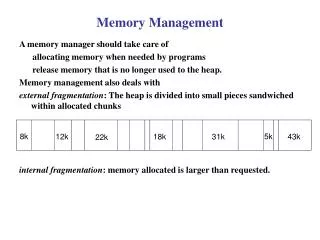
8K 12K 22K Last allocated block (14K) 18K 8K 6K Allocated block Free block 14K 36K Before Dynamic Partitioning Placement Algorithm 8K 12K Allocate 18K First Fit Next Fit Best Fit 6K 2K 8K 6K 14K 20K After
Fragmentation • External Fragmentation – total memory space exists to satisfy a request, but it is not contiguous. • Internal Fragmentation – allocated memory may be slightly larger than requested memory; this size difference is memory internal to a partition, but not being used. • Reduce external fragmentation by compaction • Shuffle memory contents to place all free memory together in one large block. • Compaction is possible only if relocation is dynamic, and is done at execution time. • I/O problem • Latch job in memory while it is involved in I/O. • Do I/O only into OS buffers.
Memory Fragmentation Solution of Fragmentation • Statistical analysis shows that given N allocated blocks, another 0.5 N blocks will be lost due to fragmentation. • On average, 1/3 of memory is unusable • (50-percent rule) • Solution – Compaction. • Move allocated memory blocks so they are contiguous • Run compaction algorithm periodically • How often? • When to schedule?
P3 P1 700 K 1000 K P4 1400 K P4 P2 2000 K P5 1900 K 2000 K P3 P3 P5 2300 K 1300 K 2500 K Memory Fragmentation Memory Compaction Process Memory Time P1 600 10 P2 1000 5 P3 300 20 P4 700 8 P5 500 15 OS 400 K 2560 K
Buddy System Buddy System • Tries to allow a variety of block sizes while avoiding excess fragmentation • Blocks generally are of size 2k, for a suitable range of k • Initially, all memory is one block • All sizes are rounded up to 2s • If a block of size 2s is available, allocate it • Else find a block of size 2s+1 and split it in half to create two buddies • If two buddies are both free, combine them into a larger block • Largely replaced by paging • Seen in parallel systems and Unix kernel memory allocation
Buddy System Buddy System Example