Download
1 / 24
250 likes | 295 Views
Unravel the complexities of gene expression from RNA-Seq data. Discover the computational hurdles, assumptions, and considerations involved in analyzing sequenced reads, sequencing depths, transcript quantification, and normalization techniques.

E N D
Once sequenced the problem becomes computational Sequenced reads sequencer cells cDNA ChIP Alignment read coverage genome
Considerations and assumptions • High library complexity • #molecules in library >> #sequenced molecules • Short reads • Read length << sequenced molecule length Not all applications satisfy this: • miRNA sequencing • Small input sequencing (e.g. single cell sequencing)
Corollaries • Libraries satisfying assumptions 1 & 2 only measure relative abundance • Key quantity: # fragments sequenced for each transcript. Need to: • Which transcript generated the observed read? • Isn’t this easy? • Reads do not uniquely map • Transcripts or genes have different isoforms • Sequencing has a ~ 1% error rate • Transcripts are not uniformly sequenced
The RNA-Seq quantification problem (simple case) • Start with a set of previous gene/transcript annotations • Assume only one isoform per gene • Assume 1-1 read to transcript correspondence. (Sequencing depth) Using the Poisson approximation to the binomial We seek to maximize the likelihood of transcript frequencies given the data Which, of course has MLE
The process of RNA-Seq quantification • Sequenced reads are aligned to a reference sequence • the species genome or • its transcriptome • Transcript abundance is measured: • By counting reads mapped to each transcript (not accurate when multiple isoforms share sequence) • By solving a maximizing the likelihood of the observed mapping given transcript abundance • To compare samples counts need to be normalized • Libraries have different sequencing depth • Sample composition may be different • Most standard normalization: counts Transcripts per Million (TPM) units
The gene expression table • Genes are quantified. Each gene or isoform has: • A TPM value • A (expected) fragment count vaue • All samples were quantified in the same fashion and arranged into a table of genes (22,000) x samples (24). • Row i gives the expression of the gene i across all samples • Row j gives the expression of genes in sample j.
But, how are these quantities computed? • Start with a set of previous gene/transcript annotations • Assume Define only one isoform per gene • Assume 1-1 read to transcript correspondence. Reads (fragments) are now short, one transcript generates many fragments. Change: Transcripts of different lengths generate fragments Transcript effective length , with MLE: Model: ,
The RNA-Seq quantification problem. Isoform deconvolution Main difference: quantification involves read assignment. Our model must capture read assignment uncertainty. Parameters: Transcript relative abundance Latent variables: Fragment alignment source Observed variables: N fragment alignments, transcripts, fragment length distribution
We can estimate the insert size distribution P1 P2 Get all single isoform reconstructions Splice and compute insert distance d1 d2 Estimate insert size empirical distribution
… and use it for probabilistic read assignment Isoform 1 Isoform 2 d2 d1 Isoform 3 d1 d2 P(d > di) For methods such as MISO, Cufflinks and RSEM, it is critical to have paired-end data
The RNA-Seq quantification problem. Isoform deconvolution d2 d1 Parameters: Transcript relative abundance Latent variables: Fragment alignment source Observed variables: N fragment alignments, transcripts, fragment length distribution Probability of the fragment alignment originating from t Can be shown it is concave, and hence solvable by expectation maximization
Summary: Current quantification models are complex • In its simplest form we assume that reads can be unequivocally mapped. This allows: • Read counts distribute multinomial with rate estimated from the observed counts • When this assumption breaks, multinomial is no longer appropriate. • More general models use: • Base quality scores • Sequence mapability • Protocol biases (e.g. 3’ bias) • Sequence biases (e.g. GC) • Handling each of these involves a more complex model where reads are assigned probabilistically not only to an isoform but to a different loci
RNA-Seq libraries revisited: End-sequence libraries • Target the start or end of transcripts. • Source: End-enriched RNA • Fragmented then selected • Fragmented then enzymatically purified • Uses: • Annotation of transcriptional start sites • Annotation of 3’ UTRs • Quantification and gene expression • Depth required 3-8 mill reads • Low quality RNA samples • Single cell RNA sequencing
Analysis of counting data requires 3 broad tasks • Read mapping (alignment): Placing short reads in the genome • Quantification: • Transcript relative abundance estimation • Determining whether a gene is expressed • Normalization • Finding genes/transcripts that are differentially represented between two or more samples. • Reconstruction: Finding the regions that originated the reads
What are we normalizing? A typical replicate scatter plot
What are we normalizing? A typical replicate scatter plot
TPM normalization • Accounts for: • Differences in sequencing depth • Differences in the number of reads generated by transcripts of different length Estimated reads/fragmentsfor the gene Total reads/fragments Length of the transcript
Sample composition impacts transcript relative abundance Cell type I Cell type II Normalizing by total reads does not work well for samples with very different RNA composition
Example normalization techniques Counts for gene i in experiment j Geometric mean for that gene over ALL experiments i runs through all n genes j through all m samples kij is the observed counts for gene i in sample j sjIs the normalization constant Alders and Huber, 2010
Lets do an experiment Similar read number, one transcript many fold changed Size normalization results in 2-fold changes in all transcripts
When everything changes: Spike-ins Lovén et al, Cell 2012