Download
1 / 27
300 likes | 340 Views
Learn about the IS curve, aggregate demand, and goods market equilibrium. Explore factors shifting the IS curve with real-world examples like the Vietnam War buildup and the Fiscal Stimulus Package of 2009.

E N D
Chapter 21 The IS Curve
Preview • This chapter develops the IS schedule, which describes the relationship between real interest rates and aggregate output when the market for real goods and services is in equilibrium.
Learning Objectives • List the four components of aggregate demand (or planned expenditure). • List and describe the factors that determine the four components of aggregate demand (or planned expenditure). • Solve for the goods market equilibrium. • Describe why the IS curve slopes downward and why the economy heads to a goods market equilibrium. • List the factors that shift the IS curve and describe how they shift the IS curve.
Planned Expenditure and Aggregate Demand • Planned expenditure is the total amount of spending on domestically produced goods and services that households, businesses, the government, and foreigners want to make. • Aggregate demand is the total amount of output demanded in the economy.
Planned Expenditure and Aggregate Demand • The total quantity demanded of an economy’s output is the sum of 4 types of spending: • -Consumption expenditure (C)-Planned investment spending (I ) • -Government purchases (G ) • -Net exports (NX )
Consumption expenditure and the consumption function: The Components of Aggregate Demand
Planned Investment Spending • Fixed investment are always planned. • Inventory investment can be unplanned. • Planned investment spending • Interest rates • Expectations
Net Exports • Made up of two components: autonomous net exports and the part of net exports that is affected by changes in real interest rates • Net export function:
Government Purchases and Taxes • The government affects aggregate demand in two ways: through its purchases and taxes • Government purchases: • Government taxes:
Goods Market Equilibrium • Keynes recognized that equilibrium would occur in the economy when the total quantity of output produced in the economy equals the total amount of aggregate demand (planned expenditure). • Solving for goods market equilibrium: Aggregate Output = Consumption Expenditure + Planned Investment Spending + Government Purchases + Net Exports
Understanding the IS Curve • What the IS curve tells us: traces out the points at which the goods market is in equilibrium • Examines an equilibrium where aggregate output equals aggregate demand • Assumes fixed price level where nominal and real quantities are the same • IS curve is the relationship between equilibrium aggregate output and the interest rate.
Why the Economy Heads Toward the Equilibrium • Interest rates and planned investment spending • Negative relationship • Interest rates and net exports • Negative relationship • IS curve: the points at which the total quantity of goods produced equals the total quantity of goods demanded • Output tends to move toward points on the curve that satisfies the goods market equilibrium.
Factors that Shift the IS Curve • The IS curve shifts whenever there is a change in autonomous factors (factors independent of aggregate output and the real interest rate). • One example is changes in government purchases, as in Figure 2.
Figure 2Shift in the IS Curve from an Increase in Government Purchases
Application: The Vietnam War Buildup, 1964–1969 • The United States’ involvement in Vietnam began to escalate in the early 1960s. • Usually during a period when government purchases are rising rapidly, central banks raise real interest rates to keep the economy from overheating. • The Vietnam War period, however, is unusual because the Federal Reserve decided to keep real interest rates constant. Hence, this period provides an excellent example of how policymakers could make use of the IS curve analysis to inform policy.
Changes in Taxes • At any given real interest rate, a rise in taxes causes aggregate demand and hence equilibrium output to fall, thereby shifting the IS curve to the left. • Conversely, a cut in taxes at any given real interest rate increases disposable income and causes aggregate demand and equilibrium output to rise, shifting the IS curve to the right.
Figure 4Shift in the IS Curve from an Increase in Taxes • Another example of what shifts the IS curve is changes in taxes, as in Figure 4
Application: The Fiscal Stimulus Package of 2009 • In the fall of 2008, the U.S. economy was in crisis. By the time the new Obama administration had taken office, the unemployment rate had risen from 4.7% just before the recession began in December 2007 to 7.6% in January 2009. • To stimulate the economy, the Obama administration proposed a fiscal stimulus package that, when passed by Congress, included $288 billion in tax cuts for households and businesses and $499 billion in increased federal spending, including transfer payments.
Application: The Fiscal Stimulus Package of 2009 • These tax cuts and spending increases were predicted to increase aggregate demand, thereby raising the equilibrium level of aggregate output at any given real interest rate and so shifting the IS curve to the right. • Unfortunately, most of the government purchases did not kick in until after 2010, while the decline in autonomous consumption and investment were much larger than anticipated. • The fiscal stimulus was more than offset by weak consumption and investment, with the result that the aggregate demand ended up contracting rather than rising, and the IS curve did not shift to the right, as hoped.
Factors that Shift the IS Curve • Changes in autonomous spending also affect the IS curve: • Autonomous consumption • Autonomous investment spending • Autonomous net exports
Autonomous Consumption • A rise in autonomous consumption would raise aggregate demand and equilibrium output at any given interest rate, shifting the IS curve to the right. • Conversely, a decline in autonomous consumption expenditure causes aggregate demand and equilibrium output to fall, shifting the IS curve to the left.
Autonomous Investment Spending • An increase in autonomous investment spending increases equilibrium output at any given interest rate, shifting the IS curve to the right. • On the other hand, a decrease in autonomous investment spending causes aggregate demand and equilibrium output to fall, shifting the IS curve to the left.
Autonomous Net Exports • An autonomous increase in net exports leads to an increase in equilibrium output at any given interest rate and shifts the IS curve to the right. • Conversely, an autonomous fall in net exports causes aggregate demand and equilibrium output to decline, shifting the IS curve to the left.
Factors that Shift the IS Curve • Another factor that shifts the IS curve is changes in financial frictions • An increase in financial frictions, as occurred during the financial crisis of 2007-2009, raises the real cost of borrowing to firms and hence causes investment spending and aggregate demand to fall
Summary Table 1 Shifts in the IS Curve from Autonomous Changes in , , , , and