Download
1 / 30
300 likes | 337 Views
Learn about statistical models, estimation, and confidence intervals. Explore linear regression models, one-sample models, residual and standard errors, Student t-distribution, and more.

E N D
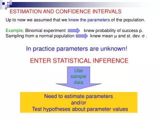
Statistical models A statistical model describes the outcome of a variable, the response variable, in terms of explanatory variables and random variation. For linear models the response is a quantitative variable. The explanatory variables describe the expected values of the response and are also called covariates or predictors. An explanatory variable is quantitative with values having an explicit numerical interpretation as in linear regression model. On the other hand, there are no explanatory variables for single variable data. The response is the measurement of variable, but there is no additional information about the measurement as in one sample model.
Model with remainder terms (technical) The response y is a function μ of explanatory variables plus a remainder term e describing the random variation. In general, let Here, μi includes the information from the explanatory variables and is a function of parameters θ1,…,θp and explanatory variable x The remainder terms e1,…,en are assumed to be independent and N(0,σ2) distributed, all with mean zero and standard deviation σ.
Linear regression model The linear regression has the size p = 2 of parameters, and (θ1,θ2) correspond to (α,β). The function f(xi;α,β) = α+β· xi determines the model where e1,…,en are independent and N(0,σ2) distributed. Or, equivalently, the model assumes that y1,…,yn are independent. The parameters of the model are α, β, and σ. The slope parameter β is the expected increment in y as x increases by one unit, whereas α is the expected value of y when x = 0. This interpretation of α does not always make biological sense as the value zero of x may be nonsense. The remainder terms e1,…,en represent the vertical deviations from the straight line. The assumption of variance homogeneity means that the typical size of these deviations is the same across all values of x.
One sample model In one sample case, there is no explanatory variable (although there could have been one such as sex or age). We assume that y1,…,yn are independent with All observations are assumed to be sampled from the same distribution. Equivalently, we may write where e1,…,en are independent and N(0,σ2) distributed. The parameters are μ and σ2, where μ is the expected value (or population mean) and σ is the average deviation from this value (or the population standard deviation).
Residual variance (technical) We get the fitted values, the residuals, and the residual sum of squares (denoted SS). The fitted value is the value we would expect for the ith observation if we repeated the experiment, and we can think of the residual ri as a “guess” for ei since ei = yi−μi. Therefore, it seems reasonable to use the residuals to estimate the variance σ2. The number n−p in the denominator is called the residual degrees of freedom, or residual df, and s2 is often referred to as the residual mean squares, the residual variance, or the mean squared error (denoted MS).
Standard error (SE) The estimate of standard deviation σ is given by the residual standard deviation s; i.e., the square root of s2. The statistical model results in the estimate of parameters θ1,…,θp. The standard deviation of the estimate is called the standard error, and given by The constant kj depends on the model and the data structure—but not on the observed data. The value of kj could be computed even before the experiment was carried out. In particular, it decreases when the sample size n increases.
Student t distribution If we replace σ with its estimate s and consider instead • Symmetry. The distribution of T is symmetric around zero, so positive and negative values are equally likely. • Dispersion. Values far from zero are more likely for T than for Z due to the extra uncertainty. This implies that the interval should be wider for the probability to be retained at 0.95. • Large samples. When the sample size increases then s is a more precise estimate of σ, and the distribution of T more closely resembles the standard normal distribution. In particular, the distribution of T should approach N(0,1) as n approaches infinity.
Student t distribution Density functions are compared for the t distribution with r = 1 degree of freedom (solid) and r = 4 degrees of freedom (dashed) as well as for N(0,1) (dotted). The probability of an interval is the area under the density curve, illustrated in the figure below.
Student t distribution It can be proven that these properties are indeed true. The distribution of T is called the t distribution with n−1 degrees of freedom and is denoted t(n−1) or tn−1, so we write The t distribution is often called Student's t distribution because the distribution result was first published in 1908 under the pseudonym “Student”. The author was a chemist, William S. Gosset, employed at the Guinness brewery in Dublin. Gosset worked with what we would today call quality control of the brewing process. Due to time constraints, small samples of 4 or 6 were used, and Gosset realized that the normal distribution was not the proper one to use. The Guinness brewery only let Gosset publish his results under pseudonym.
The t distribution table Density for the t10 distribution. The 95% quantile is 1.812, as illustrated by the gray region which has area 0.95. The 97.5% quantile is 2.228, illustrated by the dashed region with area 0.975.
The t distribution table The following table shows the 95% and 97.5% quantiles for the t distribution for a few selected degrees of freedom for illustration. The quantiles are denoted t0.95,r and t0.975,r as illustrated for r = 10. For data analyses where other degrees of freedom are in order, you should look up the relevant quantiles in a statistical table, called the t distribution table.
Confidence interval: one sample model In one sample case let y1,…,yn be independent and N(μ,σ2) distributed. The estimate of parameters μ and σ2 are given by and hence the standard error of the parameter μ is given by By standardization we obtain
Confidence interval: one sample model If we denote the 97.5% quantile in the tdistribution by t0.975,n−1, then If we move around terms in order to isolate μ, we get Therefore, the interval includes the true parameter value μ with a probability of 95%. The interval is called a 95% confidence interval for μ.
Confidence interval in general Using the estimate of μ and its corresponding standard error, we can write the 95% confidence interval for μ by That is, the confidence interval has the form In general, confidence intervals for any parameter in a statistical model can be constructed in this way.
Confidence interval in general If we repeated the experiment or data collection procedure many times and computed the interval then 95% of those intervals would include the true value of μ. We have drawn 50 samples of size 10 with μ = 0, and for each of these 50 samples we have computed and plotted the confidence interval. The true value μ = 0 is included in the confidence interval 95% of the time. The 75% confidence interval for μ is given by The 75% confidence intervals are more narrow such that the true value is excluded more often, with a probability of 25% rather than 5%. This reflects that our confidence in the 75% confidence interval is smaller compared to the 95% confidence interval.
Confidence interval in general Confidence intervals for 50 simulated data generated for the true value μ = 0. Each shows 95% confidence intervals of size n = 10, 75% confidence intervals of size n = 10, and 95% confidence intervals of size n = 40, respectively.
Confidence interval in general The true value μ0 is either inside the interval or it is not, but we will never know. We can, however, interpret the values in the confidence interval as the values for which it is reasonable to believe that they could have generated the data. If we use 95% confidence intervals, • the probability of observing data for which the corresponding confidence interval includes μ0 is 95% • the probability of observing data for which the corresponding confidence interval does not include μ0 is 5% As a standard phrase we may say that the 95% confidence interval includes those values that are in agreement with the data on the 95% confidence level.
Summary: Confidence interval Construction. In general we denote the confidence level 1−α, such that 95% and 90% confidence intervals corresponds to α = 0.05 and α = 0.10, respectively. The relevant t quantile is 1−α/2, assigning probability α/2 to the right. Then (1−α)-confidence interval for a parameter θ is of the form where r is the degrees of freedom. Interpretation.The 1−α confidence interval includes the values of θ for which it is reasonable, at confidence degree 1−α, to believe that they could have generated the data. If we repeated the experiment many times then a fraction 1−α of the corresponding confidence intervals would include the true value θ.
SE for linear regression (technical) In the linear regression model, the estimate of parameters are given by In order to simplify formulas, define SSx as the denominator in the definition. The standard errors are given by where
SE for the predicted (technical) In regression analysis we often seek to estimate the prediction for a particular value of x. Let x0 be such an x-value of interest. The predicted value of the response is denoted μ0; that is, μ0 = α+β· x0. It is estimated by The predicted value has the standard error
Example: Stearic acid and digestibility Researchers examined the digestibility of fat with different levels of stearic acid. The average digestibility percent was measured for nine different levels of stearic acid proportion. Data are shown in the table below, where x represents stearic acid and y is digestibility measured in percent.
Example: Stearic acid and digestibility Consider the linear regression model which describes the association between the level of stearic acid and digestibility. The residual sum of square SSe = 61.7645 is used to calculate
Example: Stearic acid and digestibility There are n = 9 observations and p = 2 parameters. Thus, we need quantiles from the t distribution with 7 degrees of freedom. Since t0.95,7 = 1.895 and t0.975,7 = 2.365, we compute the 90% and the 95% confidence interval for the slope parameter β. Hence, decrements between 0.76 and 1.11 percentage points of the digestibility per unit increment of stearic acid level are in agreement with the data on the 90% confidence level.
Example: Stearic acid and digestibility If we consider a stearic acid level of x0 = 20%, then we will expect a digestibility percentage of which has standard error The 95% confidence interval for μ0 is given by In conclusion, the predicted values of digestibility percentage corresponding to a stearic acid level of 20% between 75.2 and 80.5 are in accordance with the data on the 90% confidence level.
Example: Stearic acid and digestibility We can calculate the 95% confidence interval for the expected digestibility percentage for other values of the stearic acid level.
Example: Parasite counts for salmons An experiment with two difference salmon stocks, from River Conon in Scotland and from River Ätran in Sweden, was carried out as follows. The statistical model for the salmon data is given by where g(i) is either “Ätran” or “Conon” and e1,…,e26 are from N(0,σ2). In other words, Ätran observations are N(αÄtran,σ2) distributed, and Conon observations are N(αConon,σ2) distributed
Example: Parasite counts for salmons We can compute the group means and the residual standard deviation. The difference in parasite counts is estimated by with a standard error of The 95% confidence interval for the difference is given by We see that the data is not in accordance with a difference of zero between the stock means. Thus, the data suggests that Ätran salmons are more susceptible than Conon salmons to parasites during an infection.
Unpaired samples with different SD’s • Assume that the observations y1, . . . , yn are independent and come from • two different groups, group 1 and group 2. Observations from group 1 • are assumed to be N(μ1, σ21 ) and observations from group 2 are • assumed to be N(μ2, σ22 ). The standard error is estimated by The 95% confidence interval for the difference is given by with degrees of freedom
Unpaired samples with different SD’s • Under the assumption of different SD’s we get the standard error • For the degrees of freedom we get r = 22.9. So the 95% confidence interval for the difference becomes • almost the same as before, where the SD’s are assumed to be the same for the two stocks. In general the results based on the assumption of equal SD’s are quite robust as long as the samples are roughly of the same size and not too small.