Download
1 / 57
570 likes | 597 Views
Learn how marketers and economists measure consumer demand through techniques such as surveys, experiments, and historical data analysis. Understand the concepts of linear and log-linear demand functions, elasticities, and coefficient of determination.

E N D
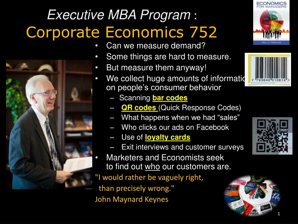
Executive MBA Program :Corporate Economics 752 • Can we measure demand? • Some things are hard to measure. • But measure them anyway! • We collect huge amounts of information on people’s consumer behavior • Scanning bar codes • QR codes (Quick Response Codes) • What happens when we had “sales” • Who clicks our ads on Facebook • Use of loyalty cards • Exit interviews and customer surveys • Marketers and Economists seek to find out who our customers are. "I would rather be vaguely right, than precisely wrong." John Maynard Keynes
Consumer Demand and BehaviorChapter 4 Ninja Marketing Who is pregnant?– if you knew before other firms, how would you use this information? Target - used baby shower registry info; who bought baby name books; and purchase of 25 maternity related items to make a “pregnancy prediction” score on its customers. Send coupons, email messages, etc. Creepy? Yes. Well, they mixed in baby coupons with others coupons to mask their knowledge.
Techniques for Estimating Consumer Demand New Products have no historical data – so surveys can assess interest in new ideas. Common Survey Problems • Sample bias--telephone, magazine • Biased questions-- • advocacy surveys • Ambiguous questions • Respondents may lie on questionnaires Survey Research Center of U. of Mich. does repeat surveys of households on Big Ticket items (Autos) Surveys of Spending Plans
information on demand • Consumer Surveys • ask a sample of consumers their attitudes • panel data of a sample of customers • Consumer Clinics • experimental groups try to emulate a market (Hawthorne effect, see youtube links),Laboratory experiments • Market Experiments • get demand info by trying different prices, store audit, in store pricing experiments • scanning data, uncontrolled studies of actual purchases • Historical Data • what happened in the past is guide to the future https://www.youtube.com/watch?v=W7RHjwmVGhs\ https://www.youtube.com/watch?v=EEwCWR5Vkpw Videos on the Hawthorne effect
Just Plot Historical Data quantity Q • Look at the relationship of price and quantity over time • Then plot it Q = a + b P + • Plotting is subject to difference of opinion on “best fitting line” Slope isb a 19 18 16 15 14 17 13 Price P
Simple Linear RegressionQuick Review from Layth’s Class OLS -- ordinary least squares Q • Qt = a + b Pt + t Time subscripts & error term Find “best fitting” line t = Qt - a - b Pt t 2= [Qt - a - b Pt] 2 • mint 2 = [Qt - a - b Pt] 2 • Solution: b = Cov(Q,P) / Var(P) a = mean(Q) - b•mean(P) a b is slope _ Q _ P
Functional Forms: 1. Linear Demand Functions • Linear Form Q = a + b •P + c •I • The effect of each variable is constant • The effect of each variable is independent of other variables • Elasticities • Price elasticity is: E P =b•P /Q =DQ/DP)(P/Q) • Income elasticity is: E I = c•I /Q=DQ/DI) (I/Q)
2. Multiplicativeor Log Linear • MultiplicativeQ = A • P b • Ic • The effect of each variable depends on all the other variables and is not constant • It is log linear or also called double logged Ln Q = a + b•Ln P + c•Ln I • The price elasticity is b • The income elasticity is c • Proof: E P = DQ/DP) ( P/Q ) =(b A•P b-1•I c) (P/ A• P b • I c) =b
R2The Coefficient of Determinationa.k.a. “The R-Square” Q • R-square -- % of variation in the dependent variable that is explained by the independent variables • Ratio of RSS [Qt -Qt] 2 TSS [Qt - Qt] 2 . • As more variables are included, R-square rises • Adjusted R-square, however, can decline – see page 98 for Adj R2 ^ Qt Qt ^ [Qt -Qt] 2 _ Q ^ = __ _ P
Different samples would yield different coefficients Test the hypothesis that the coefficient equals zero Ho: b = 0 Ha: b 0 RULE: If absolute value of the estimated t >Critical-t, then REJECT Ho. It’s significant! estimated t = (b - 0) / b critical t Large Samples, critical t2 N > 30 Small Samples, critical t is on Student’s t-table D.F. = # observations, minus number of independent variables, minus one. N < 30 T-tests
Table 4.2: Price & Advertising Variable Coeff Std Error T-statistic Intercept 116.2 24.6 4.7 Price -1.308 .013 -10.1 Advert. 11.2 2.8 4.0 N=12 R-square=.961 Q= 116.2 – 1.3 Price + 11.2 Advert = 100.2 at P=70 and Advert = 6. Find elasticities at P=70 and Advert = 6.7 EP = slope * P/Q = -1.3 (70/100.2) = -.908 Q: Is the product elastic or inelastic? Should we raise the price?
Multiple Regression on Campus Apartments Linear Q = a + bP + cA + dDPrice, Advertising, & Distance to Campus from ten apartments complexes each with 100 units. R-square = .79, and Adj R-square = .69 Coeff Std Err T-value Intercept 135.15 20.65 6.54 Price - .14 .06 - 2.41 Advertising .54 .85 0.85 Distance - 5.78 1.26 - 4.61 • What is the estimated demand curve? • Q = 135.15 - .14 Price + .54 Advertising – 5.78 Distance • Does this make economic sense? Which are significant? • They all make sense, but only Price and Distance appear significant. • Find the price elasticity and suggest if rents should be raised. • Demand elasticity of -1.11 is elastic. Raising rents will decrease apartment revenue. • Find all of the elasticities. Average Price = $420 per occupant. Average Quantity Rented = 53.1; Average advertising = $8; Average Distance = 2 miles Price Elasticity = - .14 (420) / 53.1 = - 1.11 Advertising Elasticity = .54(8) / 53.1 = .081 Distance Elasticity = -5.78(2)/53.1 = .218
A Log Linear Demand For Campus Apartments Dependent Variable: Ln Q Variable Coefficient Std Error T-value Constant 14 7 2 Log P -1.15 .5 -2.3 Log A .05 .06 0.83 Log D -.19 .04 -4.75 R-sqr = .567 Adj R-sqr = .545 N=10 • Do the signs of the coefficients make economic sense? • Which form, linear or log linear fit the data better? • What are the three elasticities?
Auto Demand: Tables 4.3 & 4.4 • 23 variables from search cost, quality perception, to socioeconomic variables • Explains only 26% of variation but most variables are significant. • Price elasticity of whole market -.87 • Cross price elasticity +.82 (vs. Asian or European cars) • Income elasticity +1.7 • Characterized the auto market. Pages 105 & 106
Coffee-mate by Carnation • Brand names matter • Market for coffee non-dairy additives • Price elasticity -2.01 • In-ad coupons and special prices were effective • Store displays were not statistically significant • Increase ads for Cremora added to sales of Coffee-mate. Can you explain that! 16 Oz Size
Evaporated Milk by Carnation • Used in pies, soups, sauces and also used in coffee sometimes. • Store label substitutes used more by younger, less affluent customers. • Purchased only once per year (in the fall). • Price elasticity of -2.03 for Carnation • Pet Evaporated Milk EP = -.88 • Positive cross price elasticity
Computer Analysis of Firm Data, 10 regions of the country SALES = a + b1 Advertising + b2 Price + b3 Income Dependent Variable: SALES Multiple R = .899 Squared multiple R = .790 Adjusted multiple R = .684 Std error of estimate = 17.417 N = 10 Variable Coefficient Std Error T-stat p Constant 310.245 95.075 3.263 .017 Advertising 0.008 0.204 0.308 .971 Price -12.202 4.582 -2.663 .037 Income 2.667 3.160 0.847 .429
1. Write as an equation: Sales = 310.245+.008 Advertising - 12.202 Price + 2.667 Income 2. Do the coefficients make economic sense? Yes -- higher advertising & income increase sales, but higher price reduces sales. 3. What is the critical t-value? d.f. = 6, so critical t = 2.447 4. Are the coefficients statistically significant (at the .05 significance level)? Only Constant & Price are significant
Regression Models for Forecasting • Can we use the regression output for forecasting? Yup! • Firm can forecast for one region: sales for a region with Advertising = 100, Price = $10, and Income = 21, and output on slide 66. • Answer: • Sales = 310.245+.008 {100} - 12.202 {10} + 2.667 {21} = 251.96 2 (17.417) • Gives the approx. 95% confidence interval
Log Linear Example Dependent Variable: Ln Q Variable Coefficient Std Error T-value Constant 14 7 2 Log P -1.2 .5 -2.4 Log I .30 .6 0.5 R-sqr = .567 Adj R-sqr = .545 N=34 • Do the signs of the coefficients make economic sense? • CHARACTERIZE the demand curve, using estimates of the relevant elasticities.
Nonlinear Forms • Semi-logarithmic transformations. Sometimes taking the logarithm of the dependent variable or an independent variable improves the R2. Examples are: • log Y = + ß·X. • Here, Y grows exponentially at rate ß in X; that is, ß percent growth per period. • Y = + ß·log X. Here, Y doubles each time X increases by the square of X. Ln Y = .01 + .05X Y X
Reciprocal Transformations • The relationship between variables may be inverse. Sometimes taking the reciprocal of a variable improves the fit of the regression as in the example: • Y = + ß·(1/X) • shapes can be: • declining slowly • if beta positive • rising slowly • if beta negative E.g., Y = 500 + 2 ( 1/X) Y X
Polynomials • Quadratic, cubic, and higher degree polynomial relationships are common in business and economics. • Profit and revenue are cubic functions of output. • Average cost is a quadratic function, as it is U-shaped • Total cost is a cubic function, as it is S-shaped TC = ·Q + ß·Q2 + ·Q3is a cubic total cost function. • If higher order polynomials improve the R-square, then the added complexity may be worth it.
Discussion Time – Yeah! • Ask, “what I don’t get is…” or • Using economics, please explain why we do what we do.
Executive MBA Program :Corporate Economics 752 • Chapter 5. Time and motion studies. • Examination of ways to reduce mistakes and increase efficiency • Drive-through windows • How to speed up the process • Increase accuracy • Monitors with selections listed • Suggested items to purchase • These are the things of import to McDonald’s, Burger King, Arby’s, Dunkin’ Donuts, and Starbucks. • Or, go delivery like freaky fast Jimmy John’s. • Or, Jeff Bezos's drones.
Production and Cost Analysis in the Short RunChapter 5 • Our business classes presume production occurs in a firm • We can & do produce things at home • Suppose all goods produced in households • Limited by size of household • Suppose there exist some economies of scale in organizational size
Let two households merge: • If more productive, then other households will emulate them. • Four households merge • Iftrue for 2 households, why not true if 2 million households merged? • So problems arise as the size of the collective grows • Less Personal Incentives • Who is in Charge? • Disagreements & Conflict Resolution Issues
Entrepreneurship • Synonym is CONTRACTOR • contractor monitors production • hires labor at fixed rates • purchases materials • receives the residual • This is a firm-- contractor - entrepreneur • 87% of all production by corporations • remaining 13% in proprietorships & other
Competing Views onFirm Behavior & Conflicts Over Ownership 1. Standard View a. Firms are owned by shareholders, hence transfers of ownership are easy, and potentially perpetual. b. Firms provide limited liabilityup to amount invested. Note that as firm's merge, they dilute the effectiveness of the limited liability. (Partnerships & Proprietorships don't have this protection). c. Firms allow separation of management and ownership.
d. The objective for firm managers is to maximize the present value of the stream of profits: PV = [ Profitst /(1+rt)t ] COMMENT:This approach works well for relationships between rival firms. It is less help dealing with conflicts of interest within firms. 2. Principal-Agent Theoryconflicts reduced through appropriate incentives. • The agents (managers) may wish to maximize leisure and minimize risk, • whereas the principal (shareholders) may wish hard work and high risk-return investments.
The Free Rider Problem • Example:an employee knows that working hard helps the whole firm, and helps himself only a little. Why not let the other workers be grinds and just take it easy (be a free rider)? • Principal-Agent problems may lead to: •Risk Avoidance in Managers • Managers have Short Time Horizons • Sales Maximization • High Levels of Social Amenities at the Work Site • Satisficing or Sufficing Behavior • COMMENT: Competition among managers and competition among firms in acquisition tend to limit non-profit maximizing behavior.
Attempt is to align manager's interests with shareholders by: profit incentives, ownership positions, or options. • Creation of profit centers and transfer prices to create rewards and incentives. • But ownership of a little stock does not eliminate the free rider problem, that a lost $1 of profit "hurts" a partial owner only a tiny bit. • COMMENT: This approach helps explain the existence of bonuses and transfer pricing, but it doesn't explain why some firms are vertically integrated and others contract-out many steps in production.
Example:Vertical integration via merger(Boise Cascade buys OfficeMax) OfficeMax/Office Depot stores transfer price Boise Cascade paper division • Who wants a low transfer price? • Who wants a high transfer price? • Leads to Internal Conflict
3. Transaction Cost Economics • Ronald Coase-- use of the price system is costly • Use of internal price systems are also costly. • When do we integrate? • When the costs are lower than contracting through separate firms. • When do we spin off tasks? • When the costs are low for explicit contracts • Few steps involved • Easy to observe quality of workmanship
4. Nexus of Contracts Management Shareholders Employees Bondholders Customers Government Suppliers All parties have “interests” in the firm FIRM
The "owners" of a firm are broadly defined as those who have relationships with the firm via contracts. • This includes bondholders, management, and employees. • The residual claimant (shareholders) have only a liquidation lien on what is left over. • Most managers and employees think of themselves as "their" firm. They wear lapel pins or shirts with their firm’s logo on it. • COMMENT: All four views of corporate life are correct in different settings.
Production Functions • Q = f ( K, L ) for two input case, with K as Fixed • If not at maximum output for a set of inputs: we suffer X-inefficiency (perhaps due to lack of motivation or spirit to excel). • Short Run Production Functions: • Max output, from a n y set of inputs • Q = f ( X1, X2, X3, X4, ... ) FIXED IN SRVARIABLE IN SR _
Average Product = Q / L • output per labor • Marginal Product =Q / L • output attributable to last unit of labor applied • Similar to profit functions, the Peak of MP occurs before the Peak of average product • When MP = AP, we’re at the peak of the AP curve
Short Run Production Function Example Marginal Product Average Product See also Table 5.1 page 119 1 2 3 4 5 6
When MP > AP, then AP is RISING • IF YOUR MARGINAL GRADE IS HIGHER THAN YOUR AVERAGE GRADE POINT AVERAGE, THEN YOUR G.P.A. IS RISING • When MP < AP, then AP is FALLING • IF THE MARGINAL WEIGHT ADDED TO A TEAM IS LESS THAN AVERAGE WEIGHT, THEN AVERAGE TEAM, WEIGHT DECLINES • When MP = AP, then AP is at its MAX • IF THE NEW HIRE IS JUST AS EFFICIENT AS THE AVERAGE EMPLOYEE, THEN AVERAGE PRODUCTIVITY DOESN’T CHANGE
Law of Diminishing Returns INCREASES IN ONE FACTOR OF PRODUCTION, HOLDING ONE OR OTHER FACTORS FIXED, AFTER SOME POINT, MARGINAL PRODUCT DIMINISHES. Total Output A SHORT RUN LAW point of diminishing returns input
The Stages of Production(Bakers and Cupcakes Stage 1 Stage 2 Stage 3 Q Stage 1 • MP is rising or falling • AP is RISING • You’d expand L in this region. Stage 2 • MP is declining • AP is declining • Usual region to produce Stage 3 • MP is negative. • Don’t go here! Inflection point L AP MP L
Fill in the following table Number of Bakers Total Output MP AP 5 500 unknown 100 6 ---- ----- 105 7 740 ----- --- 8 ---- 105 ---
Fill in the following table Number of Bakers Total Output MP AP 5 500 unknown 100 6 630130 105 7 740 110105.71 8 845105 105.63
Optimal Use of Inputs • If there are two inputs, efficiency is best served if the MPA / PA = MPB / PBwhere MPA and MPBare marginal products of inputs A and B, and PA and PB are input prices of A and B, respectively. • E.g.: MPA= 20 and MPB = 30, and PA= $5 and PB = $10, then we are NOT efficient as we get 4 units per dollar of A and only 3 for B. • So, reduce use of B by one and lose 3 items, but spend that $10 on A and get 8 items. More for less. Cool man! RULE: Find where the MP per dollar in each input is equal • If the marginal product per dollar in A is greater than the marginal product per dollar in B, use more A.
Two primary components of cost: a. input prices -- amount spent to purchase inputs b. productivity -- how productive are those inputs SHORT RUN COST FUNCTIONS 1. TC = FC + VC fixed & variable costs 2. ATC = AFC + AVC = FC/Q + VC/Q
Short Run Cost Graphs MC ATC 3. 1. AVC AFC AFC Q Q MCintersects lowest point of AVC and lowest point of ATC. When MC < AVC, AVC declines When MC > AVC, AVC rises 2. AVC Q
Typically use TIME SERIES data of cost Cubic Total Cost Functions TC = C0 + C1 Q + C2 Q2 + C3Q3 TC Q Q 2 Q3 5000 20 400 8000 4233 15 225 3375 4980 19 361 6859 REGR c1 1 c2 c3 c4 EstimatingShort Run Cost Functions Minitab Output: Predictor Coeff StdErr T-value Constant 1000 300 3.3 Q 50 20 2.5 Q-squared -10 2.5 -4.0 Q-cubed 1 2.0 0.5 R-square = .93 Adj R-square = .90 N = 38
Empirical Evidence on Shapes of Cost Curves See page 133 on shapes. • Econometric – such as the cubic one just examined. • Structured Survey Questions – how much variable, how much fixed costs, etc. • Constant versus Rising Marginal Costs – varies by industries • Implications for Managers – Knowing costs can bring profits. • Ex: Sony and Akio Morita. If average cost is U-shaped, then making more can lower cost per unit. He did.