Download

1 / 65
660 likes | 852 Views
UET Multiprocessor Scheduling Problems. Nan Zang nzang@cs.ucsd.edu. Overview of the paper. Introduction Classification Complexity results for Pm | prec, p j = 1 | C max Algorithms for Pk | prec, p j = 1 | C max Future research directions and conclusions. Scheduling.

E N D
UET MultiprocessorScheduling Problems Nan Zang nzang@cs.ucsd.edu
Overview of the paper • Introduction • Classification • Complexity results for Pm | prec, pj = 1 | Cmax • Algorithms for Pk | prec, pj = 1 | Cmax • Future research directions and conclusions Nan Zang
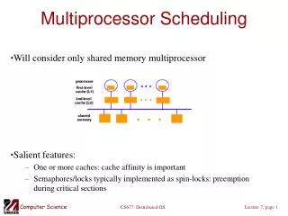
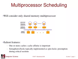
Scheduling • Scheduling concerns optimal allocation of scarce resources to activities. • For example Class scheduling problems • Courses • Classrooms • Teachers Nan Zang
Problem notation (1) • A set of n jobs J = { J1, J2, ……, Jn} The execution time of the job Jj is p(Jj). • A set of processors P = {P1 , P2, ……} • Schedule Specify which job should be executed by which processor at what time. • Objective Optimize one or more performance criteria Nan Zang
Problem Notation (2) • αdescribes the processor environment Number of processors, speed, … • β provides the job characteristics release time, precedence constraints, preemption,… • γ represents the objective function to be optimized The finishing time of the last job (makespan) The total waiting time of the jobs 3-field notation α|β|γ (Graham et al.) Nan Zang
Job Characteristics • Release time (rj) - earliest time at which job Jj can start processing. - available job • Preemption (prmp) - jobs can be interrupted during processing. • Precedence constraints (prec) - before certain jobs are allowed to start processing, one or more jobs first have to be completed. - a ready job Nan Zang
Precedence constraints (prec) Definition • Successor • Predecessor • Immediate successor • Immediate predecessor • Transitive Reduction Before certain jobs are allowed to start processing, one or more jobs first have to be completed. Nan Zang
Precedence constraints (prec) Definition • Successor • Predecessor • Immediate successor • Immediate predecessor • Transitive Reduction One or more job have to be completed before another job is allowed to start processing. Nan Zang
Precedence constraints (prec) Definition • Successor • Predecessor • Immediate successor • Immediate predecessor • Transitive Reduction One or more job have to be completed before another job is allowed to start processing. Nan Zang
Special precedence constraints (1) • In-tree (Out-tree) • In-forest (Out-forest) • Opposing forest • Interval orders • Quasi-interval orders • Over-interval orders • Series-parallel orders • Level orders Nan Zang
In-tree Out-tree Opposing forest In-forest Special precedence constraints (2) Out-forest Nan Zang
UET scheduling problem formal definition Pm| prec, pj = 1 | Cmax (m≥1) • Processor Environment • m identical processors are in the system. • Job characteristics • Precedence constraints are given by a precedence graph; • Preemption is not allowed; • The release time of all the jobs is 0. • Objective function • Cmax : the time the last job finishes execution. ( If cj denotes the finishing time of Jj in a schedule S, ) Nan Zang
Slot 1 Slot 2 P1 P2 P3 Time axis Gantt Chart A Gantt chart indicates the time each job spends in execution, as well as the processor on which it executes Nan Zang
Overview of the paper • Introduction • Classification • Complexity results for Pm | prec, pj = 1 | Cmax • Algorithms for Pk | prec, pj = 1 | Cmax • Future research directions and conclusions Nan Zang
Classification Due to the number of processors • Number of processors is a variable (m) Pm | prec, pj = 1 | Cmax • Number of processors is a constant (k) Pk | prec, pj = 1 | Cmax Nan Zang
Classification Due to the number of processors • Number of processors is a variable (m) Pm| prec, pj = 1 | Cmax • Number of processors is a constant (k) Pk| prec, pj = 1 | Cmax Nan Zang
Pm| prec, pj = 1 | Cmax (1) Theorem 1 Pm| prec, pj = 1 | Cmax is NP-complete. • Ullman (1976) 3SAT ≤ Pm | prec, pj = 1 | Cmax 2. Lenstra and Rinooy Kan (1978) k-clique ≤ Pm| prec, pj = 1 | Cmax • Corollary 1.1 • The problem of determining the existence of a schedule with Cmax ≤3 for the problem • Pm| prec, pj = 1 | Cmax is NP-complete. Nan Zang
Pm| prec, pj = 1 | Cmax (2) Mayr (1985) • Theorem 2 Pm | pj =1, SP | Cmax is NP-complete. SP: Series - parallel • Theorem 3 Pm | pj =1, OF | Cmax is NP-complete. OF: Opposing - forest Nan Zang
a b c d SP and OF • Series-parallel orders Does NOT have a substructure isomorphic to Fig 1. • Opposing-forest orders Is a disjoint union of in-tree orders and out-tree orders. Fig 1 Fig 2: Opposing forest Nan Zang
Conclusion on Pm| prec, pj = 1 | Cmax • 3SAT is reducible to the corresponding scheduling problem. • m is a function of the number of clauses in the 3SAT problem. • Results and techniques do not hold for the case Pk | prec, pj = 1 | Cmax Nan Zang
Classification • Number of processors is a variable (m) Pm | prec, pj = 1 | Cmax • Number of processors is a constant (k) Pk | prec, pj = 1 | Cmax Nan Zang
Optimal Schedule for Pk | prec, pj = 1 | Cmax • The complexity of Pk | prec, pj = 1 | Cmax is open. • 8th problem in Garey and Johnson’s open problems list.(1979) • One of the three problems remaining unsolved in that list • If k = 2, P2 | prec, pj = 1 | Cmax is solvable in polynomial time. • Fujii, Kasami and Ninomiya (1969) • Coffman and Graham (1972) • For any fixed k, when the precedence graph is restricted to certain special forms, Pk | prec, pj = 1 | Cmax turns out to be solvable in polynomial time. • In-tree, Out-tree, Opposing-forest, Interval orders… Nan Zang
Special precedence constraints • In-tree (Out-tree) • In-forest (Out-forest) • Opposing forest • Interval orders • Quasi-interval orders • Over-interval orders • Level orders Nan Zang
Algorithms for Pk | prec, pj = 1 | Cmax • List scheduling policies • Graham’s list algorithm • HLF algorithm • MSF algorithm • CG algorithm • FKN algorithm (Matching algorithm) • Merge algorithm Nan Zang
Algorithms for Pk | prec, pj = 1 | Cmax • List scheduling policies • Graham’s list algorithm • HLF algorithm • MSF algorithm • CG algorithm • FKN algorithm (Matching algorithm) • Merge algorithm Nan Zang
List scheduling policies (1) • Set up a priority list L of jobs. • When a processor is idle, assign the first ready job to the processor and remove it from the list L. Nan Zang
Algorithms for Pk | prec, pj = 1 | Cmax • List scheduling policies • Graham’s list algorithm • HLF algorithm • MSF algorithm • CG algorithm • FKN algorithm (Matching algorithm) • Merge algorithm Nan Zang
Graham’s list algorithm • Graham first analyzed the performance of the simplest list scheduling algorithm. • List scheduling algorithm with an arbitrary job list is called Graham’s list algorithm. • Approximation ratio for Pk | prec, pj = 1 | Cmax δ = 2-1/k. (Tight!) • Approximation ratio is δ if for each input instance, the makespan produced by the algorithm is at most δ times of the optimal makespan. Nan Zang
Algorithms for Pk| prec, pj = 1 | Cmax • List scheduling policies • Graham’s list algorithm • HLF algorithm • MSF algorithm • CG algorithm • FKN algorithm (Matching algorithm) • Merge algorithm Nan Zang
HLF algorithm (1) • T. C. Hu (1961) • Critical Path algorithm or Hu’s algorithm • Algorithm • Assign a level h to each job. • If job has no successors, h(j) equals 1. • Otherwise, h(j) equals one plus the maximum level of its immediate successors. • Set up a priority list L by nonincreasing order of the jobs’ levels. • Execute the list scheduling policy on this level based priority list L. Nan Zang
Level 3 Level 2 Level 1 HLF algorithm (2) 3 3 3 3 2 2 1 1 1 1 1 1 1 Nan Zang
HLF algorithm (3) • Time complexity O(|V|+|E|) (|V| is the number of jobs and |E| is the number of edges in the precedence graph) • Theorem 4 (Hu, 1961) The HLF algorithm is optimal for Pk | pj = 1 , in-tree (out-tree) | Cmax. • Corollary 4.1 The HLF algorithm is optimal for Pk | pj = 1 , in-forest (out-forest) | Cmax. Nan Zang
HLF algorithm (4) • N.F. Chen & C.L. Liu (1975) The approximation ratio of HLF algorithm for the problem with general precedence constraints: If k = 2, δHLF ≤ 4/3. If k ≥ 3, δHLF ≤ 2 – 1/(k-1). Tight! Nan Zang
Algorithms for Pk | prec, pj = 1 | Cmax • List scheduling policies • Graham’s list algorithm • HLF algorithm • MSF algorithm • CG algorithm • FKN algorithm (Matching algorithm) • Merge algorithm Nan Zang
MSF algorithm (1) • Algorithm: • Set up a priority list L by nonincreasing order of the jobs’ successors numbers. (i.e. the job having more successors should have a higher priority in L than the job having fewer successors) • Execute the list scheduling policy based on this priority list L. Nan Zang
MSF algorithm (2) 2 2 2 7 1 6 0 0 0 0 0 0 0 7 6 2 2 2 1 0 0 0 0 0 0 0 Nan Zang
MSF algorithm (3) • Time complexity O(|V|+|E|) • Theorem 5(Papadimitriou and Yannakakis, 1979) The MSF algorithm is optimal for Pk | pj = 1, interval | Cmax. • Theorem 6 (Moukrim, 1999) The MSF algorithm is optimal for Pk | pj = 1, quasi-interval | Cmax. Nan Zang
a b a b c b c d a b a c e d d e e d c Special precedence constraints • Interval orders Does NOT have a substructure isomorphic to Fig 1. • Quasi – interval orders Does NOT have a substructure isomorphic to TYPE I, II or III. Type II Fig 1 Type III Type I Nan Zang
Algorithms for Pk | prec, pj = 1 | Cmax • List scheduling policies • Graham’s list algorithm • HLF algorithm • MSF algorithm • CG algorithm • FKN algorithm (Matching algorithm) • Merge algorithm Nan Zang
CG algorithm (1) • Coffman and Graham (1972) • An optimal algorithm for P2 | prec, pj = 1 | Cmax. • Best approximation algorithm known for Pk | prec, pj = 1 | Cmax, where k ≥ 3. Nan Zang
CG algorithm (2) • Definitions • Let IS(Jj) denote the immediate successors set of Jj. • A job is ready to label, if all its immediate successors are labeled and it has not been labeled yet. • N(Jj) denotes the decreasing sequence of integers formed by ordering of the set { label (Ji) | Ji IS(Jj) }. • Let label(Jj) be an integer label assigned to Jj. Nan Zang
CG algorithm (3) • Assign a label to each job: • Choose an arbitrary task Jk such that IS(Jk) = 0, and define label(Jk) to be 1 • for i 2 to n do • R be the set of jobs that are ready to label. • Let J* be the task in R such that N(J*) is lexicographically smaller than N(J) for all J in R • Let label(J*) i end for 2. Construct a list of jobs L = {Jn, Jn-1,…, J2, J1} according to the decreasing order of the labels of the jobs. 3. Execute the list scheduling policy on this priority list L. Nan Zang
13 12 11 10 9 8 7 6 5 4 3 2 1 CG algorithm (4) N(J10)= N(J11)=N(J12)=(8) 10 11 12 13 N(J8)=(7,6,5,4,3,2) 8 9 N(J9)=(1) 1 2 3 4 5 6 7 Nan Zang
CG algorithm (4) 10 11 12 13 8 9 1 2 3 4 5 6 7 13 12 11 10 9 8 7 6 5 4 3 2 1 Nan Zang
CG algorithm (5) • Time complexity O(|V|+|E|) • Theorem 5(Coffman and Graham, 1972) The CG algorithm is optimal for P2 | prec, pj = 1| Cmax. • Theorem 6 (Moukrim, 2005) The CG algorithm is optimal for Pk | pj = 1, over-interval | Cmax. Nan Zang
a b c b a b a c d e d e e d c Special precedence constraints • Quasi – interval orders Does NOT have a substructure isomorphic to TYPE I, II or III. • Over – interval orders Does NOT have a substructure isomorphic to TYPE I or II. Type II Type I Type III Nan Zang
CG algorithm (6) The performance of CG algorithm when k≥3 • Lam and Sethi (1978) δCG ≤ 2 – 2/k • Braschi and Trystram (1994) Cmax(S) ≤ (2 – 2/k) Cmax(S*) – (k – 2 – odd(k))/k (tight!) Note: S is a CG schedule. S* is an optimal schedule. If k is an odd, odd(k):=1; otherwise, odd(k):=0. Nan Zang
List Scheduling Policy Conclusions • List scheduling policies • Graham’s list algorithm • HLF algorithm • MSF algorithm • CG algorithm • Property • easy to implement • extended to the problem Pm | prec, pj = 1| Cmax • Research directions: • Allow priority lists to depend on the number k of processors. Nan Zang
Algorithms for Pk | prec, pj = 1 | Cmax • List scheduling policy algorithm • Graham’s list algorithm • HLF algorithm • MSF algorithm • CG algorithm • FKN algorithm (Matching algorithm) • Merge algorithm Nan Zang
FKN algorithm (1) • Fujii, Kasami and Ninomiya (1969) • First optimal algorithm for P2 | prec, pj = 1 | Cmax. • Basic Idea • Find a minimum partition of the jobs • There are at most two jobs in each set. • The pair of jobs in the same set can be executed together. • Make a valid schedule according to a particular order of the partition. (Some clever swap work needed!) • The length of the result schedule = value of the min partition • Can be solved by some maximum matching algorithm. Nan Zang