Download
1 / 18
180 likes | 324 Views
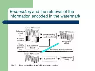
Embedding and the retrieval of the information encoded in the watermark. WATERMARKING 3D MODELS ALGORITHM. SELECTING THE LOCATION. Step 1: We consider a vertex where 3D coordinates are given by the vector V i , from then 3D model.

E N D
Embedding and the retrieval of the information encoded in the watermark
SELECTING THE LOCATION Step 1: We consider a vertex where 3D coordinates are given by the vector Vi , from then 3D model. We define its neighbourhood as all vertices connected to it :
SELECTING THE LOCATION Step2: We calculate the distance from a vertex to its neighbourhood as :
SELECTING THE LOCATION Step3: Sorting Di . We select those vertices which have their Di smaller than a threshold T.
EMBEDDING THE WATERMARK(the first approach ) Step 4: We derive the ellipsoid which roughly models the neighbourhood of Vi. The center of this ellipsoid is given by :
SELECTING THE LOCATION Step5: Let us consider that we have an watermark code of B bits. The chosen vertices are split in sets of B vertices. The vertices from each set are ranked with respect to the distance between the neighbouring ellipsoids centers.
EMBEDDING THE WATERMARK (the first approach ) Step 1: We calculate the normal Nj at each vertex from the neighbourhood , VjN(j). Qi is given by averaging the orientations of all surface normals from that neighbourhood:
EMBEDDING THE WATERMARK (the first approach ) Step 2: The two plances are located on both side , at equal distance from the center ui. The distance is derived as the variance of the local neighbourhood distances projected along the direction of Qi.
EMBEDDING THE WATERMARK(the first approach ) Step 3: In the case when embedding a 1 bit we project the vertex Vi along the direction of Qi inside the volume define by the bounding planes such that :
EMBEDDING THE WATERMARK(the second approach) Step 1: We can calculate the shape of the ellipsoid on the same set of locations.
EMBEDDING THE WATERMARK (the second approach) Step 2: The ellipsoid which locally describes the vertices in the neighbourhood of Vi forms a bounding volume which is modelled by : where x is a vector located inside the bounding volume described by (ui , Si) and characterising N(Vi) , and K is a normalization factor.
EMBEDDING THE WATERMARK (the second approach) Step 3: When embedding a 1 bit , the vertex Vi is projected along the direction of the line Viui, inside the bounding ellipsoid . In this case we have : where:
DETECTING THE WATERMARK A sequence of bits is retrieved from the graphical object when checking the geometrical relations : OR
EXPERIMENTAL RESULTS The watermarked “dog” model using bounding planes for embedding the watermark. There are 54 vertices where we can embed watermarks for dog.
EXPERIMENTAL RESULTS The watermarked “screwdriver” model using ellipsoids for embedding the watermark. There are 43 possible bit holder vertices for the “screwdriver”.
EXPERIMENTAL RESULTS In order to measure the distortion brought to the object by watermarking we evaluate the mean square error (MSE) between the vertices composing the original and the watermarked object. Where M is the total number of vertices which make up the graphical object.
EXPERIMENTAL RESULTS The MSE for the “dog” is The MSE for the “screwdriver” is