Lecture 4. Importance of being small

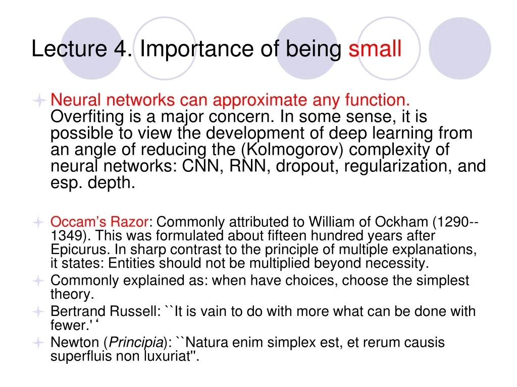
1. Lecture 4. Importance of being small • Neural networks can approximate any function. Overfiting is a major concern. In some sense, it is possible to view the development of deep learning from an angle of reducing the (Kolmogorov) complexity of neural networks: CNN, RNN, dropout, regularization, and esp. depth. • Occam’s Razor: Commonly attributed to William of Ockham (1290--1349). This was formulated about fifteen hundred years after Epicurus. In sharp contrast to the principle of multiple explanations, it states: Entities should not be multiplied beyond necessity. • Commonly explained as: when have choices, choose the simplest theory. • Bertrand Russell: ``It is vain to do with more what can be done with fewer.'‘ • Newton (Principia): ``Natura enim simplex est, et rerum causis superfluis non luxuriat''.

2. Example. Inferring a deterministic finite automaton (DFA) • A DFA accepts: 1, 111, 11111, 1111111; and rejects: 11, 1111, 111111. What is it? • There are actually infinitely many DFAs satisfying these data. • The first DFA makes a nontrivial inductive inference, the 2nd does not. • The 2nd one “over fits” the data, cannot make further predictions. 1 1 1 1 1 1 1

3. Exampe. History of Science • Maxwell's (1831-1879)'s equations say that: • (a) An oscillating magnetic field gives rise to an oscillating electric field; • (b) an oscillating electric field gives rise to an oscillating magnetic field. Item (a) was known from M. Faraday's experiments. However (b) is a theoretical inference by Maxwell and his aesthetic appreciation of simplicity. The existence of such electromagnetic waves was demonstrated by the experiments of H. Hertz in 1888, 8 years after Maxwell's death, and this opened the new field of radio communication. Maxwell's theory is even relativistically invariant. This was long before Einstein’s special relativity. As a matter of fact, it is even likely that Maxwell's theory influenced Einstein’s 1905 paper on relativity which was actually titled `On the electrodynamics of moving bodies'. • J. Kemeny, a former assistant to Einstein, explains the transition from the special theory to the general theory of relativity: At the time, there were no new facts that failed to be explained by the special theory of relativity. Einstein was purely motivated by his conviction that the special theory was not the simplest theory which can explain all the observed facts. Reducing the number of variables obviously simplifies a theory. By the requirement of general covariance Einstein succeeded in replacing the previous ‘gravitational mass' and `inertial mass' by a single concept. • Double helix vs triple helix --- 1953, Watson & Crick

4. Bayesian Inference • Bayes Formula: P(H|D) = P(D|H)P(H)/P(D) • By Occam’s razor, P(H)=2-K(H), (smallest most likely). • Take -log, maximize P(H|D) becomes minimize: -logP(D|H) + K(H) (modulo logP(D), constant). where • -log P(D|H) is the coding length of D given H. • K(H) is the smallest description of model H (Kolmogorov complexity of H).

5. Note • The next 4 pages are only for theoretically oriented students to read. • Here is an informal statement: given data (positive and negative examples drawn from distribution D), if you find a model M that agrees with the data, and size of M is polynomially smaller than the data, then with high probability (according to D) , M is correct with a small number of errors.

6. PAC Learning (L. Valiant, 1983) • Fix a distribution for the sample space (P(v) for each v in sample space). A concept class C is pac-learnable (probably approximately correct learnable) iff there exists a learning algorithm A such that, for each f in C and  (0 <  < 1), algorithm A halts in a polynomial number of steps and examples, and outputs a concept h in C which satisfies the following. With probability at least 1- , Σf(v) ≠ h (v) P(v) < 

7. Simplicity means understanding • We will prove that given a set of positive and negative data, any consistent concept of size `reasonably' shorter than the size of data is an `approximately' correct concept with high probability. That is, if one finds a shorter representation of data, then one learns. The shorter the conjecture is, the more efficiently it explains the data, hence the more precise the future prediction. • Let α < 1, β ≥ 1, m be the number of examples, and s be the length (in number of bits) of the smallest concept in C consistent with the examples. An Occam algorithm is a polynomial time algorithm which finds a hypothesis h in C consistent with the examples and satisfying K(h) ≤ sβ mα

8. Occam Razor Theorem(Blummer, Ehrenfeucht, Haussler, Warmuth,This kolmogorov complexity version is from Li-Tromp-Vitanyi, IPL) Theorem. A concept class C is polynomially pac-learnable if there is an Occam algorithm for it. Proof. Fix an error tolerance  (0 < <1). Choose m such that m ≥ max { (2sβ/ )1/(1- α) , 2/  log 1/  }. I.e. m is a polynomial in s and 1/ . Let S be a set of r concepts, and let f be one of them. Claim The probability that any concept h in S satisfies P(f ≠ h) ≥  and is consistent with m independent examples of f is less than (1-  )m r. Proof: Let Eh be the event that hypothesis h agrees with all m examples of f. If P(h ≠ f ) ≥ , then h is a bad hypothesis. That is, h and f disagree with probability at least  on a random example. The set of bad hypotheses is denoted by B. Since the m examples of f are independent, P( Eh ) ≤ (1-  )m . Since there are at most r bad hypotheses, P( Uh in B Eh) ≤ (1- )m r. QED (claim)

9. Proof of the theorem continues The postulated Occam algorithm finds a hypothesis of Kolmogorov complexity at most sβmα. The number r of hypotheses of this complexity satisfies log r ≤ sβmα . By assumption on m, r ≤ (1-  )-m/ 2 (Use  < - log (1- ) <  /(1- ) for 0 <  <1). Using the claim, the probability of producing a hypothesis with error larger than  is less than (1 -  )m r ≤ (1-  )m/2 < . The last inequality is by substituting m. QED