Chapter 6 Regression Algorithms in Data Mining
300 likes | 458 Views
Chapter 6 Regression Algorithms in Data Mining. Fit data Time-series data: Forecast Other data: Predict. Contents. Describes OLS (ordinary least square) regression and Logistic regression Describes linear discriminant analysis and centroid discriminant analysis

Chapter 6 Regression Algorithms in Data Mining
E N D
Presentation Transcript
Chapter 6Regression Algorithms in Data Mining Fit data Time-series data: Forecast Other data: Predict
Contents • Describes OLS (ordinary least square) regression and Logistic regression • Describes linear discriminant analysis and centroid discriminant analysis • Demonstrates techniques on small data sets • Reviews the real applications of each model • Shows the application of models to larger data sets
Use in Data Mining • Telecommunication Industry, turnover (churn) • One of major analytic models for classification problem. • Linear regression • The standard –ordinaryleast squares regression • Can use for discriminant analysis • Can apply stepwise regression • Nonlinear regression • More complex (but less reliable) data fitting • Logistic regression • When data are categorical (usually binary)
OLS Regression • Uses intercept and slope coefficients (b) to minimize squared error terms over all i observations • Fits the data with a linear model • Time-series data: • Observations over past periods • Best fit line (in terms of minimizing sum of squared errors)
Regression Output R2 : 0.987 Intercept: 0.642 t=0.286 P=0.776 Week: 5.086 t=53.27 P=0 Requests = 0.642 + 5.086*Week
Example R2 SSE SST
Regression Tests • FIT: • SSE – sum of squared errors • Synonym: SSR – sum of squared residuals • R2–proportion explained by model • Adjusted R2– adjusts calculation to penalize for number of independent variables • Significance • F-test - test of overall model significance • t-test - test of significant difference between model coefficient & zero • P – probability that the coefficient is zero • (or at least the other side of zero from the coefficient) See page. 103
Regression Model Tests • SSE (sum of squared errors) • For each observation, subtract model value from observed, square difference, total over all observations • By itself means nothing • Can compare across models (lower is better) • Can use to evaluate proportion of variance in data explained by model • R2 • Ratio of explained squared dependent variable values (MSR) to sum of squares (SST) • SST = MSR plus SSE • 0 ≤ R2 ≤ 1 See page. 104
Multiple Regression • Can include more than one independent variable • Trade-off: • Too many variables – many spurious, overlapping information • Too few variables – miss important content • Adding variables will always increase R2 • Adjusted R2penalizes for additional independent variables
Example: Hiring Data • Dependent Variable – Sales • Independent Variables: • Years of Education • College GPA • Age • Gender • College Degree See page. 104-105
Regression Model Sales = 269025 -17148*YrsEd P = 0.175 -7172*GPA P = 0.812 +4331*Age P = 0.116 -23581*Male P = 0.266 +31001*Degree P = 0.450 R2 = 0.252 Adj R2 = -0.015 Weak model, no significant at 0.10
Improved Regression Model Sales = 173284 - 9991*YrsEd P = 0.098* +3537*Age P = 0.141 -18730*Male P = 0.328 R2 = 0.218 Adj R2 = 0.070
Logistic Regression • Data often ordinal or nominal • Regression based on continuous numbers not appropriate • Need dummy variables • Binary – either are or are not • LOGISTIC REGRESSION (probability of either 1 or 0) • Two or more categories • DISCRIMINANT ANALYSIS (perform regression for each outcome; pick one that fit’s best)
Logistic Regression • For dependent variables that are nominal or ordinal • Probability of acceptance of • case i to class j • Sigmoidal function • (in English, an S curve from 0 to 1)
Insurance Claim Model Fraud = 81.824 -2.778 * Age P = 0.789 -75.893 * Male P = 0.758 + 0.017 * Claim P = 0.757 -36.648 * Tickets P = 0.824 + 6.914 * Prior P = 0.935 -29.362 * Atty Smith P = 0.776 Can get probability by running score through logistic formula See page. 107~109
Linear Discriminant Analysis • Group objects into predetermined set of outcome classes • Regression one means of performing discriminant analysis • 2 groups: find cutoff for regression score • More than 2 groups: multiple cutoffs
Centroid Method (NOT regression) • Binary data • Divide training set into two groups by binary outcome • Standardize data to remove scales • Identify means for each independent variable by group (the CENTROID) • Calculate distance function
Discriminant Analysis with RegressionStandardized data, Binary outcomes Intercept 0.430 P = 0.670 Age -0.421 P = 0.671 Gender 0.333 P = 0.733 Claim -0.648 P = 0.469 Tickets 0.584 P = 0.566 Prior Claims -1.091 P = 0.399 Attorney 0.573 P = 0.607 R2 = 0.804 Cutoff average of group averages: 0.429
Case: Stepwise Regression • Stepwise Regression • Automatic selection of independent variables • Look at F scores of simple regressions • Add variable with greatest F statistic • Check partial F scores for adding each variable not in model • Delete variables no longer significant • If no external variables significant, quit • Considered inferior to selection of variables by experts
Credit Card Bankruptcy PredictionFoster & Stine (2004), Journal of the American Statistical Association • Data on 244,000 credit card accounts • 12-month period • 1 percent default • Cost of granting loan that defaults almost $5,000 • Cost of denying loan that would have paid about $50
Data Treatment • Divided observations into 5 groups • Used one for training • Any smaller would have problems due to insufficient default cases • Used 80% of data for detailed testing • Regression performed better than C5 model • Even though C5 used costs, regression didn’t
Summary • Regression a basic classical model • Many forms • Logistic regression very useful in data mining • Often have binary outcomes • Also can use on categorical data • Can use for discriminant analysis • To classify