Understanding Simple Regression: Concepts, Methods, and Applications
This chapter introduces the fundamentals of simple regression, exploring the relationship between random variables and the strength of their correlation. It discusses covariance and correlation coefficients, the method of least squares, and the significance of linear relationships through t-tests. The chapter also covers essential concepts like prediction intervals, confidence intervals, and regression coefficients. Practical examples, including the relationship between shoe length and height, illustrate these concepts to enhance understanding. Key focus areas include linear modeling and assumptions relevant to accurate predictions.

Understanding Simple Regression: Concepts, Methods, and Applications
E N D
Presentation Transcript
6.1 - Introduction Fundamental questions • Is there a relationship between two random variables and how strong is it? • Can we predict the value of one if we know the value of the other? Example • The author had ten of his students measure their shoe length and height
6.2 – Covariance and Correlation Definition 6.2.1 Let and be two random variables with respective means and . The covariance of and is Alternatively,
Correlation Coefficient Definition 6.2.2 Let and be random variables with standard deviations and , respectively. The correlation coefficient of and is Theorem 6.2.2
Sample Correlation Coefficient Definition 6.2.3 The sample correlation coefficient of n pairs of data values is Alternatively,
Sample Correlation Coefficient r measures the strength of a linear relationship
Bivariate Normal Distribution Definition 6.2.4 Let Two variables X and Y are said to have a bivariate normal distribution if their joint p.d.f. is
Bivariate Normal Distribution Theorem 6.2.3 Two random variables and with a bivariate normal distribution are independent if and only if .
T-test of T-test of for Bivariate Random Variables Purpose: To test the null hypothesis H0: where and have a bivariate normal distribution. • Test statistic • Critical value: t-score with degrees of freedom
Example 6.2.4 For the shoe length vs height data, , • Test the claim that H0: H1: • Test statistic
Example 6.2.4 • Critical value: • Critical region: • P-value = twice the region to the right of which is 0 • Reject H0 Final conclusion: • There is a statistically significant linear relationship between shoe length and height.
6.3 – Method of Least-Squares We want to find and that minimize
Example 6.3.1 Suppose a crime scene investigator finds a shoe print outside a window that measures 11.25 in long and would like to estimate the height of the person who made the print Cautions • If there is no linear correlation, do not use a linear regression equation to make predictions • Only use a linear regression equation to make predictions within the range of the x-values of the data
6.4 – The Simple Linear Model Definition 6.4.1 Two random variables and are said to be described by a simple linear model if where and are constants and is a random variable independent of that is where is a constant.
Residuals Definition 6.4.2 For a set of data the residuals are where and are the least-squares estimates of m and b as calculated in Section 6.3 • Observed values of
Standard Error of Estimate Definition 6.4.3 Let and be described by a simple linear model. The standard error of estimate is • An unbiased estimate of , the variance of
Prediction Interval Definition 6.4.4 Let and be described by a simple linear model. Given a value of , say , a prediction interval estimate for the corresponding value of is where , the margin of error is and is a critical t-value with d.f.
Confidence Interval for Definition 6.4.5 Let X and Y be described by a simple linear model . A confidence interval estimate of is where the margin of error is and is a critical t-value with d.f.
T-Test of the Slope Let and be described by a simple linear model . To test the null hypothesis H0: , the test statistic is the critical value is a t-score with degrees of freedom, and the P-value is the area under the corresponding density curve.
6.5 – Sums of Squares and ANOVA Variation
Coefficient of Determination • The square of the sample correlation coefficient Interpretation • “The proportion of the total variation in the -values from explained (or accounted for) by the regression equation.”
F-Test of the Slope Let X and Y be described by a simple linear model . To test the hypotheses H0: vs. H1: , the test statistic is The critical value is The P-value is the area under the corresponding density curve to the right of the test statistic.
6.6 – Nonlinear Regression Example: and are described by • Use the data below to estimate and • is linear with respect to • “Transform” the -values
Example 6.6.1 • People/physician () • Male life expectancy () (World Almanac Book of Facts, 1992, Pharos Books) • Fit Power and Exponential models to the data
6.7 – Multiple Regression Goal: Predict the value of a variable in terms of two or more other variables • – response variable • – predictor variables Assume a relation of the form • Use software to estimate coefficients
Example Predict Selling Price in terms of Area, Acres, and Bedrooms
Outputs Coefficients: Yield the multiple regression equation Standard error: Use to calculate confidence interval estimate of the coefficients where is a critical t-value with d.f.
Outputs t Stat: Test statistic for the hypotheses H0: , H1: in the presence of the other predictor variables • Small P-value indicates that the variable is “statistically significant”
ANOVA Results F – Test statistic for the hypotheses H0: , H1: at least one is not 0 Significance F– Corresponding P-value • Measures the “overall significance” of the set of predictor variables • Small P-value: The set is “statistically significant”
Regression Statistics Multiple R – Multiple regression equivalent of the sample correlation coefficient r R Squared – Multiple coefficient of determination
Regression Statistics Adjusted R Square – Calculated with the formula • The higher the value, the better the overall quality of the model Standard Error – Estimate of the standard deviation of the random variable in the multiple regression model • Also called the standard error of estimate
Which Set of Variables is “Best?” • Very complicated to answer • A very simple approach: • Compare , Adjusted , and P-values • Area and Acres are “best”