Download
1 / 23
240 likes | 378 Views
Explore methods like Golden Section Search, Parabolic Interpolation, Newton's Method, and Conjugate Gradient for solving optimization problems. Learn about constraints, local properties, steepest descent, and simulated annealing.

E N D
Optimization Problems • Solution of equations can be formulated as an optimization problem, e.g., density functional theory (DFT) in electronic structure, Lagrangian mechanics, etc • Minimization with constraints – operations research (linear programming, traveling salesman problem, etc), max entropy with a given energy, …
General Consideration • Use function values only, or use function values and its derivatives • Storage of O(N) or O(N2) • With constraints or no constraints • Choice of methods
Bracketing and Search in 1D Bracket a minimum means that for given a < b < c, we have f(b) < f(a), and f(b) < f(c). There is a minimum in the interval (a,c). c a b
How accurate can we locate a minimum? • Let b a minimum of function f(x),Taylor expanding around b, we have • The best we can do is when the second correction term reaches machine epsilon comparing to the function value, so
Golden Section Search x • Choose x such that the ratio of intervals [a,b] to [b,c] is the same as [a,x] to [x,b]. Remove [a,x] if f[x] > f[b], or remove [b,c] if f[x] < f[b]. • The asymptotic limit of the ratio is the Golden mean c a b
Parabolic Interpolation & Brent’s Method Brent’s method combines parabolic interpolation with Golden section search, with some complicated bookkeeping. See NR, page 404-405 for details.
Minimization as a root-finding problem • Let’s derivative dF(x)/dx = f(x), then minimizing (or maximizing) F is the same as finding zero of f, i.e., f(x) = 0. • Newton method: approximate curve as a straight line.
Deriving Newton Iteration • Let the current value be xn and zero is approximately located at xn+1, using Taylor expansion • Solving for xn+1, we get
Convergence in Newton Iteration • Let x be the exact root, xi is the value in i-th iteration, and εi=xi-x is the error, then • Rate of convergence: (Quadratic convergence)
Strategy in Higher Dimensions • Starting from a point P and a direction n, find the minimum on the line P + n, i.e., do a 1D minimization of y()=f(P+n) • Replace P by P + minn, choose another direction n’ and repeat step 1. The trick and variation of the algorithms are on chosen n.
Local Properties near Minimum • Let P be some point of interest which is at the origin x=0. Taylor expansion gives • Minimizing f is the same as solving the equation T for transpose of a matrix
Search along Coordinate Directions Search minimum along x direction, followed by search minimum along y direction, and so on. Such method takes a very large number of steps to converge. The curved loops represent f(x,y) = const.
Steepest Descent Search in the direction with the largest decrease, i.e., n = -f Constant f contour line (surface) is perpendicular to n, because df = dxf = 0. The current search direction n and next search direction are orthogonal, because for minimum we have y’() = df(P+n)/d = nTf|P+n = 0 n’ nT n’ = 0 n
Conjugate Condition Make a linear coordinate transformation, such that contour is circular and (search) vectors are orthogonal n1T A n2 = 0
Conjugate Gradient Method • Start with steepest descent direction n0 = g0 = -f(x0), find new minimum x1 • Build the next search direction n1 from g0 and g1 = -f(x1), such that n0An1 = 0 • Repeat step 2 iteratively to find nj (a Gram-Schmidt orthogonalization process). The result is a set of N vectors (in N dimensions) niTAnj = 0
Conjugate Gradient Algorithm • Initialize n0 = g0 = -f(x0), i = 0, • Find that minimizes f(xi+ni), let xi+1 =xi+ni • Compute new negative gradient gi+1 = -f(xi+1) • Compute • Update new search direction as ni+1 = gi+1 + ini; ++i, go to 2 (Fletcher-Reeves)
Simulated Annealing • To minimize f(x), we make random change to x by the following rule: • Set T a large value, decrease as we go • Metropolis algorithm: make local change from x to x’. If f decreases, accept the change, otherwise, accept only with a small probability r = exp[-(f(x’)-f(x))/T]. This is done by comparing r with a random number 0 < ξ < 1.
Traveling Salesman Problem Beijing Tokyo Shanghai Taipei Hong Kong Kuala Lumpur Find shortest path that cycles through each city exactly once. Singapore
Problem set 7 • Suppose that the function is given by the quadratic form f=(1/2)xTAx, where A is a symmetric and positive definite matrix. Find a linear transform to x so that in the new coordinate system, the function becomes f = (1/2)|y|2, y = Ux [i.e., the contour is exactly circular or spherical]. More precisely, give a computational procedure for U. If two vectors in the new system are orthogonal, y1Ty2=0, what does it mean in the original system? • We’ll discuss the conjugate gradient method in some more detail following the paper: http://www.cs.cmu.edu/~quake-papers/painless-conjugate-gradient.pdf