Profit Maximization Chapter 8
This chapter explores the fundamentals of perfectly competitive markets, focusing on key assumptions such as price-taking behavior, product homogeneity, and unrestricted market entry and exit. It analyzes how firms, viewed as price takers, determine profit-maximizing output by equating marginal revenue and marginal cost. The concepts of total revenue and total cost are also discussed, exploring their implications for short-run profits and losses. Visibility into firm behavior in competitive settings, such as revenue maximization and the decision to operate at a loss, is provided throughout the chapter.

Profit Maximization Chapter 8
E N D
Presentation Transcript
PERFECTLY COMPETITIVE MARKETS • The model of perfect competition rests on three basic assumptions: (1) price taking, (2) product homogeneity, and (3) free entry and exit. Price Taking Because each individual firm sells a sufficiently small proportion of total market output, its decisions have no impact on market price. price taker Firm that has no influence over market price and thus takes the price as given.
Product Homogeneity When the products of all of the firms in a market are perfectly substitutable with one another—that is, when they are homogeneous—no firm can raise the price of its product above the price of other firms without losing most or all of its business. free entry (or exit) Condition under which there are no special costs that make it difficult for a firm to enter (or exit) an industry. When Is a Market Highly Competitive? Because firms can implicitly or explicitly collude in setting prices, the presence of many firms is not sufficient for an industry to approximate perfect competition. Conversely, the presence of only a few firms in a market does not rule out competitive behavior.
Profit Maximization • Do firms maximize profits? • Managers in firms may be concerned with other objectives • Revenue maximization • Revenue growth • Dividend maximization • Short-run profit maximization (due to bonus or promotion incentive) • Could be at expense of long run profits
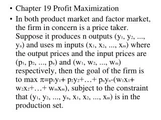
Marginal Revenue, Marginal Cost, and Profit Maximization • We can study profit maximizing output for any firm whether perfectly competitive or not • Profit () = Total Revenue - Total Cost • If q is output of the firm, then total revenue is price of the good times quantity • Total Revenue (R) = P*q Costs of production depends on output Total Cost (C) = C*q Profit for the firm, , is difference between revenue and costs
MARGINAL REVENUE, MARGINAL COST,AND PROFIT MAXIMIZATION • Revenue is curved showing that a firm can only sell more if it lowers its price • Slope in revenue curve is the marginal revenue • Change in revenue resulting from a one-unit increase in output • Slope of total cost curve is marginal cost • Additional cost of producing an additional unit of output Δπ/Δq = ΔR/Δq − ΔC/Δq = 0 MR(q) = MC(q) Profit Maximization by a Competitive Firm MC(q) = MR = P
C(q) A R(q) B q* q0 (q) Profit Maximization – Short Run Profits are maximized where MR (slope at A) and MC (slope at B) are equal Cost, Revenue, Profit ($s per year) Profits are maximized where R(q) – C(q) is maximized Output
Marginal Revenue, Marginal Cost, and Profit Maximization • Profit is maximized at the point at which an additional increment to output leaves profit unchanged
The Competitive Firm • The Competitive Firm • Price taker – market price and output determined from total market demand and supply • Market output (Q) and firm output (q) • Market demand (D) and firm demand (d) • Demand curve faced by an individual firm is a horizontal line • Firm’s sales have no effect on market price • Demand curve faced by whole market is downward sloping • Shows amount of good all consumers will purchase at different prices
The Competitive Firm • Demand curve faced by an individual firm is a horizontal line • Firm’s sales have no effect on market price • Demand curve faced by whole market is downward sloping • Shows amount of good all consumers will purchase at different prices The competitive firm’s demand Individual producer sells all units for $4 regardless of that producer’s level of output. MR = P with the horizontal demand curve For a perfectly competitive firm, profit maximizing output occurs when
MC Price Lost Profit for q2>q* 50 Lost Profit for q2>q* AR=MR=P 40 ATC AVC 30 20 10 0 1 2 3 4 5 6 7 8 9 10 11 Output q1 q* q2 A Competitive Firm q1 : MR > MC q2: MC > MR q0: MC = MR
MC Price 50 A AR=MR=P 40 ATC AVC 30 20 10 0 1 2 3 4 5 6 7 8 9 10 11 Output q1 q* q2 A Competitive Firm – Positive Profits Total Profit = ABCD Profits are determinedby output per unit times quantity Profit per unit = P-AC(q) = A to B
A Competitive Firm – Positive Profits • A firm does not have to make profits • It is possible a firm will incur losses if the P < AC for the profit maximizing quantity • Still measured by profit per unit times quantity • Profit per unit is negative (P – AC < 0) Summary of Production Decisions Profit is maximized when MC = MR If P > ATC the firm is making profits. If P < ATC the firm is making losses
MC ATC B C D P = MR A AVC q* A Competitive Firm – Losses Price At q*: MR = MC and P < ATC Losses = (P- AC) x q* or ABCD Output
Competitive Firm – Short Run Supply • When should the firm shut down? • If AVC < P < ATC the firm should continue producing in the short run • Can cover some of its variable costs and all of its fixed costs • If AVC > P < ATC the firm should shut-down. • Can not cover even its fixed costs Supply curve tells how much output will be produced at different prices Competitive firms determine quantity to produce where P = MC Firm shuts down when P < AVC Competitive firms supply curve is portion of the marginal cost curve above the AVC curve
S ATC P2 AVC P1 P = AVC q1 q2 A Competitive Firm’sShort-Run Supply Curve Price ($ per unit) The firm chooses the output level where P = MR = MC, as long as P > AVC. Supply is MC above AVC MC Output
Elasticity of Market Supply • Elasticity of Market Supply • Measures the sensitivity of industry output to market price • The percentage change in quantity supplied, Q, in response to 1-percent change in price
Producer Surplus versus Profit • Profit is revenue minus total cost (not just variable cost) • When fixed cost is positive, producer surplus is greater than profit
LMC LAC SMC SAC A D $40 P = MR C B $30 q1 q2 q3 Output Choice in the Short Run Price Output
LMC LAC SMC SAC A D $40 P = MR C B G F $30 q1 q2 q3 Output Choice in the Long Run In the long run, the plant size will be increased and output increased to q3. Long-run profit, EFGD > short run profit ABCD. Price Output
long-run competitive equilibrium • Accounting profit • Difference between firm’s revenues and direct costs • Economic profit • Difference between firm’s revenues and direct and indirect costs • Takes into account opportunity costs
long-run competitive equilibrium • Firm uses labor (L) and capital (K) with purchased capital • Accounting Profit & Economic Profit • Accounting profit: = R - wL • Economic profit: = R = wL - rK • wl = labor cost • rk = opportunity cost of capital
Long-Run Competitive Equilibrium • All firms in industry are maximizing profits • MR = MC • No firm has incentive to enter or exit industry • Earning zero economic profits • Market is in equilibrium • QD = QD
LMC LAC Economic Rent $10 $7.20 1.3 Firms Earn Zero Profit inLong-Run Equilibrium Ticket Price A team with the same cost in a larger city sells tickets for $10. Season Tickets Sales (millions)
The Industry’s Long-Run Supply Curve • To analyze long-run industry supply, will need to distinguish between three different types of industries • Constant-Cost • Increasing-Cost • Decreasing-Cost
Constant-Cost Industry Industry whose long-run supply curve is horizontal Assume a firm is initially in equilibrium Demand increases causing price to increase Individual firms increase supply Causes firms to earn positive profits in short-run Supply increases causing market price to decrease Long run equilibrium – zero economic profits
Increasing-Cost Industry • Prices of some or all inputs rises as production is expanded when demand of inputs increases • When demand increases causing prices to increase and production to increase • Firms enter the market increasing demand for inputs • Costs increase causing an upward shift in supply curves • Market supply increases but not as much
Decreasing-Cost Industry • Industry whose long-run supply curve is downward sloping • Increase in demand causes production to increase • Increase in size allows firm to take advantage of size to get inputs cheaper • Increased production may lead to better efficiencies or quantity discounts • Costs shift down and market price falls