Divide and Conquer Strategy

1. Divide and Conquer Strategy

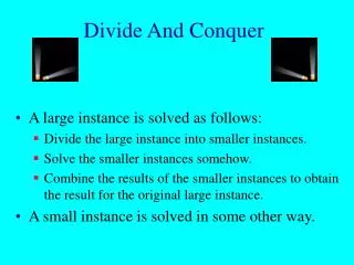
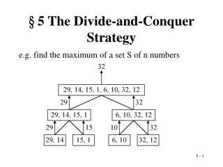
2. General Concept of Divide & Conquer • Given a function to compute on n inputs, the divide-and-conquer strategy consists of: • splitting the inputs into k distinct subsets, 1kn, yielding k subproblems. • solving these subproblems • combining the subsolutions into solution of the whole. • if the subproblems are relatively large, then divide_Conquer is applied again. • if the subproblems are small, the are solved without splitting.

3. The Divide and Conquer Algorithm Divide_Conquer(problem P) { if Small(P) return S(P); else { divide P into smaller instances P1, P2, …, Pk, k1; Apply Divide_Conquer to each of these subproblems; return Combine(Divide_Conque(P1), Divide_Conque(P2),…, Divide_Conque(Pk)); } }

4. n small otherwise Divde_Conquer recurrence relation • The computing time of Divde_Conquer is • T(n) is the time for Divde_Conquer on any input size n. • g(n) is the time to compute the answer directly (for small inputs) • f(n) is the time for dividing P and combining the solutions.

5. Three Steps of The Divide and Conquer Approach The most well known algorithm design strategy: • Divide the problem into two or more smaller subproblems. • Conquer the subproblems by solving them recursively. • Combine the solutions to the subproblems into the solutions for the original problem.

6. A Typical Divide and Conquer Case a problem of size n subproblem 1 of size n/2 subproblem 2 of size n/2 a solution to subproblem 1 a solution to subproblem 2 a solution to the original problem

7. ALGORITHM RecursiveSum(A[0..n-1]) //Input: An array A[0..n-1] of orderable elements //Output: the summation of the array elements if n > 1 return ( RecursiveSum(A[0.. n/2 – 1]) + RecursiveSum(A[n/2 .. n– 1]) ) An Example: Calculating a0 + a1 + … + an-1 Efficiency: (for n = 2k) • A(n) = 2A(n/2) + 1, n >1 • A(1) = 0;

8. the time spent on solving a subproblem of size n/b. the time spent on dividing the problem into smaller ones and combining their solutions. General Divide and Conquer recurrence The Master Theorem T(n) = aT(n/b) + f (n),where f (n)∈Θ(nk) • a < bk T(n) ∈Θ(nk) • a = bk T(n) ∈Θ(nk lg n ) • a > bk T(n) ∈Θ(nlog b a)

9. Divide and Conquer Other Examples • Sorting: mergesort and quicksort • Binary search • Matrix multiplication-Strassen’s algorithm

10. The Divide, Conquer and Combine Steps in Quicksort • Divide: Partition array A[l..r] into 2 subarrays, A[l..s-1] and A[s+1..r] such that each element of the first array is ≤A[s] and each element of the second array is ≥ A[s]. (computing the index of s is part of partition.) • Implication: A[s] will be in its final position in the sorted array. • Conquer: Sort the two subarrays A[l..s-1] and A[s+1..r] by recursive calls to quicksort • Combine: No work is needed, because A[s] is already in its correct place after the partition is done, and the two subarrays have been sorted.

11. p A[i]≤p A[i] ≥p Quicksort • Select a pivot whose value we are going to divide the sublist. (e.g., p = A[l]) • Rearrange the list so that it starts with the pivot followed by a ≤ sublist (a sublist whose elements are all smaller than or equal to the pivot) and a ≥ sublist (a sublist whose elements are all greater than or equal to the pivot ) (See algorithm Partition in section 4.2) • Exchange the pivot with the last element in the first sublist(i.e., ≤ sublist) – the pivot is now in its final position • Sort the two sublists recursively using quicksort.

12. The Quicksort Algorithm ALGORITHM Quicksort(A[l..r]) //Sorts a subarray by quicksort //Input: A subarray A[l..r] of A[0..n-1],defined by its left and right indices l and r //Output: The subarray A[l..r] sorted in nondecreasing order if l < r s  Partition (A[l..r]) // s is a split position Quicksort(A[l..s-1]) Quicksort(A[s+1..r]

13. The Partition Algorithm ALGORITHMPartition (A[l ..r]) //Partitions a subarray by using its first element as a pivot //Input: A subarray A[l..r] of A[0..n-1], defined by its left and right indices l and r (l < r) //Output: A partition of A[l..r], with the split position returned as this function’s value P A[l] i l; j  r + 1; Repeat repeat i  i + 1 until A[i]>=p //left-right scan repeat j j – 1 until A[j] <= p//right-left scan if (i < j) //need to continue with the scan swap(A[i], a[j]) until i >= j //no need to scan swap(A[l], A[j]) return j

14. Quicksort Example 15 22 13 27 12 10 20 25

15. Efficiency of Quicksort Based on whether the partitioning is balanced. • Best case: split in the middle— Θ( n log n) • T(n) = 2T(n/2) + Θ(n) //2 subproblems of sizen/2 each • Worst case: sorted array! — Θ( n2) • T(n) = T(n-1) + n+1//2 subproblems of size 0 and n-1 respectively • Average case: random arrays —Θ( n log n)

16. Binary Search – an Iterative Algorithm ALGORITHM BinarySearch(A[0..n-1], K) //Implements nonrecursive binary search //Input: An array A[0..n-1] sorted in ascending order and // a search key K //Output: An index of the array’s element that is equal to K // or –1 if there is no such element l  0, r  n – 1 while l  r do //l and r crosses over can’t find K. m (l + r) / 2 if K = A[m] return m //the key is found else if K < A[m] r m – 1 //the key is on the left half of the array else l  m + 1 // the key is on the right half of the array return -1

17. Strassen’s Matrix Multiplication • Brute-force algorithm c00 c01 a00 a01 b00 b01 = * c10 c11 a10 a11 b10 b11 a00 * b00 + a01 * b10 a00 * b01 + a01 * b11 = a10 * b00 + a11 * b10 a10 * b01 + a11 * b11 8 multiplications Efficiency class:  (n3) 4 additions

18. Strassen’s Matrix Multiplication • Strassen’s Algorithm (two 2x2 matrices) c00 c01 a00 a01 b00 b01 = * c10 c11 a10 a11 b10 b11 m1 + m4 - m5 + m7 m3 + m5 = m2 + m4 m1 + m3 - m2 + m6 • m1 = (a00 + a11) * (b00 + b11) • m2 = (a10 + a11) * b00 • m3 = a00* (b01 - b11) • m4 = a11* (b10 - b00) • m5 = (a00 + a01) * b11 • m6 = (a10 - a00) * (b00 + b01) • m7 = (a01 - a11) * (b10 + b11) 7 multiplications 18 additions

19. Strassen’s Matrix Multiplication • Two nxn matrices, where n is a power of two (What about the situations where n is not a power of two?) C00 C01 A00 A01 B00 B01 = * C10 C11 A10 A11 B10 B11 M1 + M4 - M5 + M7 M3 + M5 = M2 + M4 M1 + M3 - M2 + M6

20. Submatrices: • M1 = (A00 + A11) * (B00 + B11) • M2 = (A10 + A11) * B00 • M3 = A00* (B01 - B11) • M4 = A11* (B10 - B00) • M5 = (A00 + A01) *B11 • M6 = (A10 - A00) * (B00 + B01) • M7 = (A01 - A11) * (B10 + B11)

21. Efficiency of Strassen’s Algorithm • If n is not a power of 2, matrices can be padded with rows and columns with zeros • Number of multiplications • Number of additions • Other algorithms have improved this result, but are even more complex

22. Important Recurrence Types • Decrease-by-one recurrences • A decrease-by-one algorithm solves a problem by exploiting a relationship between a given instance of size n and a smaller size n – 1. • Example: n! • The recurrence equation for investigating the time efficiency of such algorithms typically has the form T(n) = T(n-1) + f(n) • Decrease-by-a-constant-factor recurrences • A decrease-by-a-constant algorithm solves a problem by dividing its given instance of size n into several smaller instances of size n/b, solving each of them recursively, and then, if necessary, combining the solutions to the smaller instances into a solution to the given instance. • Example: binary search. • The recurrence equation for investigating the time efficiency of such algorithms typically has the form T(n) = aT(n/b) + f (n)

23. Decrease-by-one Recurrences • One (constant) operation reduces problem size by one. T(n) = T(n-1) + c T(1) = d Solution: • A pass through input reduces problem size by one. T(n) = T(n-1) + c n T(1) = d Solution: T(n) = (n-1)c + d linear T(n) = [n(n+1)/2 – 1] c + d quadratic

24. Decrease-by-a-constant-factor recurrences – The Master Theorem T(n) = aT(n/b) + f (n),where f (n)∈Θ(nk) , k>=0 • a < bk T(n) ∈Θ(nk) • a = bk T(n) ∈Θ(nk log n ) • a > bk T(n) ∈Θ(nlog b a) • Examples: • T(n) = T(n/2) + 1 • T(n) = 2T(n/2) + n • T(n) = 3 T(n/2) + n Θ(logn) Θ(nlogn) Θ(nlog23)