Download

1 / 27
270 likes | 373 Views
Explore the general strategy of Divide and Conquer for algorithm design, examples like finding closest pair of points, Quicksort, and Matrix Multiplication Algorithm.

E N D
More examples of Divide and Conquer • Review of Divide & Conquer Concept • More examples • Finding closest pair of points • Quicksort • Matrix Multiplication Algorithm • Large Integer Multiplication
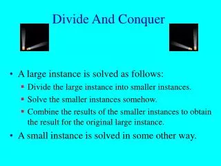
Divide and Conquer Approach • Concept: D&C is a general strategy for algorithm design. It involves three steps: (1) Divide an instance of a problem into one or more smaller instances (2) Conquer (solve) each of the smaller instances. Unless a smaller instance is sufficiently small, use recursion to do this (3) If necessary, combine the solutions to the smaller instances to obtain the solution to the original instances (e.g., Mergesort) • Approach: - Recursion (Top-down approach)
Example 1: Binary Search • Binary search in a sorted array with size n Worst case time complexity in the recursive binary search: W(n) = W(n/2) + 1 W(1) = 1 Solve the recurrence, and obtain: W(n) = lg(n) +1 (lg n)
Example 2: Closest Pair Problem • Finding the closest pair of points - Find the closest pair of points in a set of points. The set consists of points in two dimension plane - Given a set P of N points, find p, q P, such that the distance d(p, q) is minimum - Application: - traffic control systems: A system for controlling air or sea traffic might need to know which two vehicles are too close in order to detect potential collisions. - computational geometry
Brute force algorithm Input: set S of points Output: closest pair of points min_distance = infinity for each point x in S for each point y in S if x ≠ y and distance(x,y) < min_distance { min_distance = dist(x,y) closest_pair = (x,y) } Time Complexity: O(n2)
1 Dimension Closest Pair Problem • Brute-force algorithm: Find all the distances D(p, q) and find the minimum distance • Time complexity: O(n2) • 1D problem can be solved in O(nlgn) via sorting • But, sorting does not generalize to higher dimensions • Let’s develop a divide & conquer algorithm for 2D problem.
2D Closest Pair Problem • Finding the closest pair of points - The "closest pair" refers to the pair of points in the set that has the smallest Euclidean distance, Distance between points p1=(x1,y1) and p2=(x2,y2) - If there are two identical points in the set, then the closest pair distance in the set will obviously be zero.
2D Closest Pair Problem • Finding the closest pair of points - Divide: Sort the points by x-coordinate; draw vertical line to have roughly n/2 points on each side • Conquer: Find closest pair in each side recursively • Combine: Find closest pair with one point in each side • Return: best of three solutions
Example 2 Find the closest pair in a strip of width 2d Example: d= min(12, 21)
2D Closest Pair d d d = minimum (dLmin, dRmin) For each point p on the left of the dividing line, we have to compare to the distances to the points in the blue rectangle. Note there must be no point inside the blue rectangle, because d = minimum (dLmin, dRmin). Thus, for each point p, we only have to consider 6 points – 6 red circles on the blue rectangles. So, we need at most 6*n/2 distance comparisons d p d d S2 S1 Dividing Line
2D Closest Pair • Time Complexity • T(n) = 2T(n/2) + O(n) = O(nlgn) • Solve this recurrence equation yourself by applying the iterative method
Example 3: Quicksort quicksort(L) { if (length(L) < 2) return L else { pick some x in L // x is the pivot element L1 = { y in L : y < x } L2 = { y in L : y > x } L3 = { y in L : y = x } quicksort(L1) quicksort(L2) return concatenation of L1, L3, and L2 } } Source: http://www.ics.uci.edu/~eppstein/161/960118.html
Time Complexity of Quicksort • T(n) = T(n1) + T(n2) + n-1 • n1 = length of L1, n2 = length of L2 • n1 + n2 = n – 1 if all the elements in L are unique • Best case • L is divided into two halves at every recursion • T(n) = 2T(n/2) + n-1 = Θ(nlgn) • Worst case • T(n) = T(0) + T(n-1) + n-1 when the pivot is always the smallest, i.e., L is already sorted • So, T(n) = Θ(n2) • Why is it called quicksort?
How to make Quicksort efficient • Randomization • Randomly pick an element in L as the pivot • So, each item has the same probability of 1/n to be selected as the pivot • Avoid the worst case shown in the previous slide
Time Complexity of Randomized Quicksort • O(nlgn) • Proof by Induction • Refer to http://www.cs.binghamton.edu/~kang/teaching/cs333/rqsort.pdf
Example 4: Strassen’s matrix multiplication algorithm • Example: 2 by 2 matrix multiplication m1 = (a11 + a22)(b11+b22) m2 = (a21 + a22) b11 m3 = a11 (b12 – b22) m4 = a22 (b21 – b11) m5 = (a11 + a12) b22 m6 = (a21 – a11) (b11+b12) m7 = (a12 – a22)(b21 + b22)
Example 4 (cont’d) • Strassen’s matrix multiplication algorithm - partition n*n matrix into sub-matrices n/2 * n/2 (assume n is power of 2) - apply the seven basic calculations: M1 = (A11 + A22)(B11+B22) M2 = (A21 + A22) B11 M3 = A11 (B12 – B22) M4 = A22 (B21 – B11) M5 = (A11 + A12) B22 M6 = (A21 – A11) (B11+B12) M7 = (A12 – A22)(B21 + B22)
Example 4 (cont’d) • Strassen’s matrix multiplication example
Example 4 (cont’d) • What if n is no power of 2? • Add sufficient number of rows and columns of 0’s • More sophisticated approaches…
Example 4 (cont’d) • Strassen’s matrix multiplication: input: n, A, B; output: C strassen_matrix_multiply(int n, A, B, C) { divide A into A11, A12, A21, A22; divide B into B11, B12, B21, B22; strassen_matrix_multiply(n/2, A11+A22, B11+B22, M1); strassen_matrix_multiply(n/2, A21+A22, B11, M2); …… strassen_matrix_multiply(n/2, A12-A22, B21+B22, M7); Compose C11, …, C22 by M1, …, M7; }
Example 4 (cont’d) • Strassen’s matrix multiplication algorithm - Every case Time complexity Multiplications: T(n) = 7 T(n/2); T(1) = 1 T(n) = nlg7 (n2.81 ) (while brute-force approach: T(n)= (n3 ) Additions/Subtractions: T(n) = 7 T(n/2) + 18 (n/2)2 T(1) = 0 T(n) = 6nlg7– 6n2 O(n2.81 )
Example 4 (cont’d) • Strassen’s matrix multiplication algorithm - Proof of Time complexity Multiplications: T(n) = 7 T(n/2); T(1) = 1 Guess solution: T(n) = 7lgn Induction base: n=1 T(1) = 7lg1= 1 Induction hypothesis: T(n) = 7lgn Induction step: T(2n)= 7T(2n/2)=7*7lgn=7lg(2n) So the guess solution is true! Note: 7lgn = nlg7n2.18
Example 5: Large Integer Multiplication • Large digits are divided into a number of small digits - u v u = x 10m + y v = w 10m + z u v = xw 102m + (xz + wy) 10m + yz (split integer (u, v) into two equal size integers (x, y), (w, z)) e.g., 123456 = 123 *10^3 +456. 123 and 456 all have 3 digits. • Worst-case time complexity W(n) = 4 W(n/2) + cn W(n) (n2 )
Example 5 (cont’d) • In the previous solution, we need 4 multiplications xw, xz + yw, and yz; Observe that: • r = (x+y)(w+z) = xw + (xz+yw) + yz • xz + yw = r – xw – yz • So, just compute (x+y)(w+z), xw, and yz 3 multiplications • T(n) = 3T(n/2) + cn • (n1.58)
Combine the D&C algorithm with other simple algorithm • Switching point - Recursive method may not show the advantage in the case of small n as compared to the alternative algorithms - Recursive algorithm requires a fair amount of overhead. - We need to determine for what value of n it is at least as fast to call an alternative algorithm as it is to divide the instance further. - The dividing process is stopped in a certain switching point (or threshold) for recursive algorithm, and then is switched to the alternative algorithm • Example - Use the standard matrix multiplication to multiply two 2 *2 matrices
When not to use D&C algorithm • Two cases: - An instance of size n is divided into two or more instances each almost of size n, e.g., Recursive Fibonacci term is O(2n), while the iterative one is O(n) - An instance of size n is divided into almost n instances of size n/c (c is constant)