Phylogenetic Patterns: Challenges and Solutions
460 likes | 484 Views
Explore the complexities in phylogenetic analysis, from scoring characters to dealing with homoplasies and rapid radiations. Discover how molecular evolution and algorithms help reconstruct phylogenies, such as using synapomorphies and parsimony. Learn about UPGMA and its assumption of constant mutation rates. Dive into the intricate world of evolutionary patterns and solutions for analyzing data effectively.

Phylogenetic Patterns: Challenges and Solutions
E N D
Presentation Transcript
Patterns in Evolution I. Phylogenetic A. Systematics: Taxonomy and Classification B. Reconstructing Phylogenies 1. Characters 2. Trees 3. Molecular Evolution and Algorithms DNA, RNA, and protein sequence data: - thousands of characters - multiple parsimonious trees
3. Molecular Evolution and Algorithms a. Synapomorphies and parsimony Are cetaceans artiodactyls, or a sister group to the Artiodactyla?
3. Molecular Evolution and Algorithms a. Synapomorphies and parsimony Exon 7 from the gene that encodes β-casein, a protein in milk. Shared derived traits with cetaceans at positions 162, 166, 177
3. Molecular Evolution and Algorithms a. Synapomorphies and parsimony 6 changes required at these positions; 41 over entire 60 base sequence 9 changes required at these positions; 47 over entire 60 base sequence
3. Molecular Evolution and Algorithms a. Synapomorphies and parsimony 6 changes required at these positions; 41 over entire 60 base sequence 9 changes required at these positions; 47 over entire 60 base sequence
PROBLEMS WITH BASE DATA • Scoring characters-its easy if its categorical (A, C, T, G), • Homoplasies are common - both as convergence or reversal. • Ancient changes are obscured by more recent ones... A to G, then G to C, looks like it could be one change A to C. • Rapid radiations mean that branches/subgroups may not have had time to evolve their own unique synapomorphies... and we have lots of species with autapomorphies (and are thus distinct) but it is difficult to group them. • Trees of single genes may not "map" onto the phylogenetic tree among species. The loss of particular alleles may not parallel patterns of relationships. Incomplete lineage sorting
Solution: sample more genes. 70% have HC…G 30% have GC…H
PROBLEMS WITH BASE DATA • Scoring characters-its easy if its categorical (A, C, T, G), • Homoplasies are common - both as convergence or reversal. • Ancient changes are obscured by more recent ones... A to G, then G to C, looks like it could be one change A to C. • Rapid radiations mean that branches/subgroups may not have had time to evolve their own unique synapomorphies... and we have lots of species with autapomorphies (and are thus distinct) but it is difficult to group them. • Trees of single genes may not "map" onto the phylogenetic tree among species. The loss of particular alleles may not parallel patterns of relationships. • Hybridization and gene transfer - this can make populations look more similar at these loci than they really are across the whole genome. • Rates of evolution of different characters and states differ...Some are "highly conserved' and don't change much... others change dramatically. This is called mosaic evolution. This affects the "branch lengths" that are used to represent the degree of departure (or the quantified number of genetic changes in that unique lineage.
Patterns in Evolution I. Phylogenetic A. Systematics: Taxonomy and Classification B. Reconstructing Phylogenies 1. Characters 2. Trees 3. Molecular Evolution and Algorithms DNA, RNA, and protein sequence data: - thousands of characters - multiple parsimonious trees a. Synapomorphies and parsimony b. UPGMA (unweighted pair group method with arithmetic mean)
3. Molecular Evolution and Algorithms b. UPGMA - UPGMA assume constant mutation rates, and so is the simplest likelihood model. Unweighted Pair Group Method with Arithmetic Mean These are the number of differences in AA sequences between species-pairs.
3. Molecular Evolution and Algorithms b. UPGMA • The most similar sequences are those of humans and monkey (1 difference). • This difference accumulated over TWO lineages since their divergence (constant mutation) • So, the branch length of each is 1 difference / 2 branches = 0.5
1. So, we join taxa B (human) and F (monkey). 2. Then, we AVERAGE the differences between these taxa and each other taxon and reduce the matrix.... so, B differs from A by 19 AA's, and F differs from A by 18 AA's. So the average difference between A and new taxon 'BF' = 18.5 (fusion of two orange boxes into one orange box in the new and reduced matrix). (That's why this is called UPGMA - unweighted pair-group method using arithmetic averages. ASSUMES CONSTANT MUTATION RATE) B = human, F = monkey
1. So, we join taxa B (human) and F (monkey). 2. Then, we AVERAGE the differences between these taxa and each other taxon and reduce the matrix.... so, B differs from A by 19 AA's, and F differs from A by 18 AA's. So the average difference between A and new taxon 'BF' = 18.5 (fusion of two orange boxes into one orange box in the new and reduced matrix). 3. Now, in the reduced matrix, we look for the most similar pair (which is A and D = 8 diffs). We halve the difference to calculate each unique branch length (4.0) A = turtle, D = chicken
1. So, we join taxa B (human) and F (monkey). 2. Then, we AVERAGE the differences between these taxa and each other taxon and reduce the matrix.... so, B differs from A by 19 AA's, and F differs from A by 18 AA's. So the average difference between A and new taxon 'BF' = 18.5 (fusion of two orange boxes into one orange box in the new and reduced matrix). 3. Now, in the reduced matrix, we look for the most similar pair (which is A and D = 8 diffs). We halve the difference to calculate each unique branch length (4.0) 4. Repeat the averaging process
DOG Tuna Repeat until complete. Note that, having measured the branch length of B and F as 0.5, and G as 6.25, the distance from node BF to node GBF can be determined by subtraction (6.25 – 0.5 = 5.75).
3. Molecular Evolution and Algorithms b. UPGMA Here, branch lengths are equal (and additive) because averaging and constant mutation are assumed. In other models, branch lengths vary – reflecting more complex models which accept different (more realistic) substitution rates.
3. Molecular Evolution and Algorithms • Synapomorphies and parsimony • b. UPGMA • c. Branch Length Units • In the UPGMA example, the • Branch length is “mean number • of AA substitutions” in cytochrome C. • This protein has 104 AA in animals. • 2) Typically, these raw data are • Converted to “nucleotide substitutions • per site” by dividing #/length. Or, by • Multiplying this by 100, as % change. • 18 differences. • 18/104 AA = 0.173 nucleotide substitutions per site • 0.17 x 100 = 17.3 % difference
3. Molecular Evolution and Algorithms • Synapomorphies and parsimony • b. UPGMA • c. Branch Length Units • In the UPGMA example, the • Branch length is “mean number • of AA substitutions” in cytochrome C. • This protein has 104 AA in animals. • 2) Typically, these raw data are • Converted to “nucleotide substitutions • per site” by dividing #/length. Or, by • Multiplying this by 100, as % change. • 18 differences. • 18/104 AA = 0.173 nucleotide substitutions per site • 0.17 x 100 = 17.3 % difference • 3) If AA have been sequenced, data is often transformed to “minimum nucleotide substitutions” using the genetic code. Changing LEU to PRO requires at least 1 nucleotide substitution, but LEU to THR requires at least 2 substitutions.
3. Molecular Evolution and Algorithms • Synapomorphies and parsimony • b. UPGMA • c. Branch Length Units • 4) Evolutionary Modeling • The relationship between % difference • and evolutionary divergence (substitution rate) • may not be linear. • - not all differences are indicative of change; • Even 2 random sequences will only differ by 75% • (just by chance there will be the same base at 25% of sites). • - some changes are more likely than others. Transition mutations (A to G, C to T) are more likely than transversions (A to C or T). So, models incorporate a “transition/transversion ratio” (2.0, above right).
3. Molecular Evolution and Algorithms • Synapomorphies and parsimony • b. UPGMA • c. Branch Lengths • 4) Evolutionary Modeling • The relationship between % difference • and evolutionary divergence (substitution rate) • May not be linear. • - Our ability to detect change depends on existing degree of similarity. We are more likely to detect changes in sequences that are identical, than in sequences that are only 50% similar, because many changes in that case will make the sequences MORE SIMILAR. So a change in similarity from 10-12% probably represents fewer mutations, and less “genetic distance”, than observed changes from 60-62%. If sequences are 60% different, a lot of mutations in one sequence will make it more similar to the other…thus the same NET change of 2% represents MORE evolutionary change (distance).
3. Molecular Evolution and Algorithms • Synapomorphies and parsimony • b. UPGMA • c. Branch Length Units • d. Calculating Branch Lengths A a c C b B • a + b = 22 • a + c = 39 • b + c = 41 • = 2 – 3 = a – b = -2 • 5) = 1 + 4 = 2a = 20, so a = 10. • 6) The distance from A to B = 22, so b = 12, and C = 29. Hypothetical % sequence differences OR a = ((AC – BC) + AB) / 2
3. Molecular Evolution and Algorithms • Synapomorphies and parsimony • b. UPGMA • c. Branch Length Units • d. Calculating Branch Lengths Hypothetical % sequence differences among 5 taxa
3. Molecular Evolution and Algorithms • Synapomorphies and parsimony • b. UPGMA • c. Branch Length Units • d. Calculating Branch Lengths D a c 10 A,B,C b E • Hypothetical sequence differences among 5 taxa • D and E are most similar • Reduce this to a 3-point problem: D…E….ABC
3. Molecular Evolution and Algorithms • Synapomorphies and parsimony • b. UPGMA • c. Branch Length Units • d. Calculating Branch Lengths D 32.6 a c 10 A,B,C 34.6 b E • Hypothetical sequence differences among 5 taxa • D and E are most similar. • Reduce this to a 3-point problem: • Calculate average distance from D to A,B,C = 32.6 (=ac) • Calculate average distance from E to A,B,C = 34.6 (=bc)
D 32.6 a c Next, solve for ‘a’ using the formula, and solve for ‘b’ by subtraction, knowing ab = 10. 10 A,B,C 34.6 b E a = ((AC – BC) + AB) / 2 a = ((32.6 – 34.6)+10)/2 a = ((-2)+10)/2 a = 8/2 = 4 a = 4 b = 6
D 32.6 a 4 c A,B,C Now let’s recompute the complete distance matrix, finding the distance of each species to the new DE clade. A to DE = average of A-D and A-E B to DE = average of B-D and B-E C to DE = average of C-D and C-E 6 34.6 b E New matrix of distances C and DE are the closest sequences
C 40 a c 19 AB 41 b Now, reduce this to a 3-point problem: C to DE = 19 C to ‘AB’ = average of C-A and C-B = 40 AB to DE = average of A-DE and B-DE = 41 DE a = ((AC – BC) + AB) / 2
C 40 a c 19 AB 41 b Now, reduce this to a 3-point problem: C to DE = 19 C to ‘AB’ = average of C-A and C-B = 40 AB to DE = average of A-DE and B-DE = 41 DE a = ((AC – BC) + AB) / 2 Next, solve for ‘a’ using the formula, and solve for ‘b’ by subtraction, knowing ab = 19. a = ((AC – BC) + AB) / 2 a = ((40 – 41)+19))/2 a = ((-1)+19)/2 a = 18/2 = 9 a = 9 b = 10
C a 40 b is not just for that segment, it represents the complete avg. distance from the connecting node to the endpoints D and E 9 c A-B ‘10’ 41 b DE So, what do we know about the complete tree, at this point? Well, the ‘avg’ branch lengths for D (4) and E (6) = 5 And we just calculated ‘b’ as 10. So, internode length = 10 – 5 = 5. C 9 5 A-B 4 X= 5 D 6 E ‘10’
C a 40 b is not just for that segment, it represents the complete avg. distance from the connecting node to the endpoints D and E 9 c A-B ‘10’ 41 b DE So, what do we know about the complete tree, at this point? Well, the ‘avg’ branch lengths for D (4) and E (6) = 5 And we just calculated ‘b’ as 10. So, internode length = 10 – 5 = 5. And if the branch length for species C = 9, And ‘ac’, above, = 40, then the length of the AB branch = 31. C 9 31 A-B 5 4 D 6 E
So, the only thing left to compute, really, are the Branch lengths for species A and B. Recompute the complete distance matrix, combining CDE. A A to CDE = average of A-C and A-DE B to CDE = average of B-C and B-DE CDE B
So, the only thing left to compute, really, are the Branch lengths for species A and B. Recompute the complete distance matrix, combining CDE. AB is smallest value, so solve for a. a = ((AC – BC) + AB) / 2 a = ((39.5 – 41.5)+22))/2 a = ((-2)+22)/2 a = 20/2 = 10 AB = 22, so branch B = 22-10=12 A a c CDE b B
We know AB to node C = 31 We know AB(mean) = 11 So node to node = 20 C 9 A C 31 9 10 A-B 5 20 4 5 D 4 12 B D 6 6 E E
10 A WHICH was the outgroup? Lets Say C 20 12 B 6 E 5 4 D 9 C A C 9 10 20 5 4 12 B D 6 E
3. Molecular Evolution and Algorithms • Synapomorphies and parsimony • b. UPGMA • c. Branch Length Units • d. Calculating Branch Lengths • e. Neighbor Joining • Similar, but we don’t prioritize which pair we group first (like “DE”, above). Rather, we repeat the tree formation using every possible pair-wise combination, and then pick the tree with the shortest total branch lengths (most conservative evolutionary tree).
Then repeat, starting with 2 different species. Calculate total branch length.
3. Molecular Evolution and Algorithms • Synapomorphies and parsimony • b. UPGMA • c. Branch Length Units • d. Calculating Branch Lengths • e. Neighbor Joining • f. Maximum Likelihood Ratios • What evolutionary rates (in terms of transitions and tranversions, etc., are required to give us the pattern and rate (as measured in branch lengths) that we SEE? • So, different models of evolution are tested. The models are probability matrices of substitution rates between bases. • 1 – the sequence data is ‘given’ • 2 – the tree and branch lengths are calculated from this data – ‘given’ • 3 - models of evolution (changes in mutation rates) are tested. • 4 – output is the probability (‘likelihood’) of generating the data/tree with the model. • 5 – Model that generates the highest likelihood is accepted.
x x Prob.
3. Molecular Evolution and Algorithms • Synapomorphies and parsimony • b. UPGMA • c. Branch Length Units • d. Calculating Branch Lengths • e. Neighbor Joining • f. Maximum Likelihood Models • g. Bootstrapping • Gain confidence in a node by subsampling the data and creating a tree. Is the node still there? How frequently is it present in 100 or 1000 subsamples of the data set?
Randomly sample characters (in this case, base positions). Create trees. Report the frequency of a clade in these trees.
Bootstrap using entire 1100 bases of casein gene, N = 1000. Whales are within the Artiodactyla in 99% of clades. Whales are in clade with deer, hippo, cow (100%)
3. Molecular Evolution and Algorithms • Synapomorphies and parsimony • b. UPGMA • c. Branch Length Units • d. Calculating Branch Lengths • e. Maximum Likelihood Models • Neighbor Joining • g. Bootstrapping • h. Bayesian inference
3. Molecular Evolution and Algorithms • Synapomorphies and parsimony • b. UPGMA • c. Branch Length Units • d. Calculating Branch Lengths • e. Neighbor Joining • f. Maximum Likelihood Models • g. Bootstrapping • h. Bayesian inference Estimate the probability distributions (likelihoods) of slightly different trees, and estimate concordance among them for clade consensus.
3. Molecular Evolution and Algorithms • Synapomorphies and parsimony • b. UPGMA • c. Branch Length Units • d. Calculating Branch Lengths • e. Neighbor Joining • f. Maximum Likelihood Models • g. Bootstrapping • h. Baysian inference • SINE’s and LINE’s • - Short and Long interspersed sequences – transposable elements. • - Highly unlikely to end up in the same place in the genome by chance… • - Similarity is most likely a SHARED, DERIVED character.