Download
1 / 16
160 likes | 238 Views
Linear scaling fundamentals and algorithms. José M. Soler Universidad Autónoma de Madrid. Linear scaling = Order(N). CPU load. 3. ~ N. ~ N. Early 90’s. ~ 100. N (# atoms). Order-N DFT. Find density and hamiltonian (80% of code) Find “eigenvectors” and energy (20% of code)

E N D
Linear scaling fundamentals and algorithms José M. Soler Universidad Autónoma de Madrid
Linear scaling = Order(N) CPU load 3 ~ N ~ N Early 90’s ~ 100 N (# atoms)
Order-N DFT • Find density and hamiltonian (80% of code) • Find “eigenvectors” and energy (20% of code) • Iterate SCF loop • Steps 1 and 3 spared in tight-binding schemes
3 • Computational load ~ N DFT: successful but heavy • Computationally much more expensive than empirical atomic simulations • Several hundred atoms in massively parallel supercomputers
Key to O(N): locality Large system ``Divide and conquer’’ W. Yang, Phys. Rev. Lett. 66, 1438 (1992) ``Nearsightedness’’ W. Kohn, Phys. Rev. Lett. 76, 3168 (1996)
Basis sets for linear-scaling DFT • LCAO: - Gaussian based + QC machinery • G.Scuseria (GAUSSIAN), • M. Head-Gordon (Q-CHEM) • - Numerical atomic orbitals (NAO) • SIESTA • S. Kenny &. A Horsfield (PLATO) • - Gaussian with hybrid machinery • J. Hutter, M. Parrinello • Bessel functions in ovelapping spheres • P. Haynes & M. Payne • B-splines in 3D grid • D. Bowler & M. Gillan • Finite-differences (nearly O(N))J. Bernholc
x central b c b buffer buffer central buffer x’ Divide and conquer Weitao Yang (1992)
f(E) = 1/(1+eE/kT) n cn En F cn Hn Etot = Tr[ F H ] 1 ^ ^ 0 ^ ^ Emin EF Emax Fermi operator/projector Goedecker & Colombo (1994)
= 3 2 - 2 3 Etot() = H = min 1 0 -0.5 0 1 1.5 Density matrix functional Li, Nunes & Vanderbilt (1993)
Sij = < i | j > | ’k > = j | j > Sjk-1/2 EKS = k< ’k | H | ’k > = ijk Ski-1/2< i | H | j > Sjk-1/2 = Tr[ S-1 H ] Kohn-Sham EO(N) = Tr[ (2I-S) H ] Order-N ^ ^ Wannier O(N) functional • Mauri, Galli & Car, PRB 47, 9973 (1993) • Ordejon et al, PRB 48, 14646 (1993)
O(N) Non-orthogonality penalty KS Sij = ij EO(N) = EKS Order-N vs KS functionals
Chemical potential Kim, Mauri & Galli, PRB 52, 1640 (1995) • (r) = 2ij i(r) (2ij-Sij) j(r) • EO(N) = Tr[ (2I-S) H ]# states = # electron pairs • Local minima • EKMG = Tr[ (2I-S) (H-S) ]# states > # electron pairs = chemical potential (Fermi energy) Ei < |i| 0 Ei > |i| 1 Difficulties Solutions • Stability of N() Initial diagonalization • First minimization of EKMG Reuse previous solutions
i Rc rc Orbital localization i(r) = ci(r)
Convergence with localisation radius Si supercell, 512 atoms Relative Error (%) Rc (Ang)
x i x 0 2 5.37 5.37 3 1.85 8.29 1.85 = 15.34 3.14 0 = 0 1.15 0 = 0 ------- Sum 15.34 1.85 7 2.12 0 0 i y 0 2.12 3 8.29 0 4 3.14 8 1.15 Sparse vectors and matrices Restore to zero xi 0 only
Actual linear scaling c-Si supercells, single- Single Pentium III 800 MHz. 1 Gb RAM 132.000 atoms in 64 nodes