Using gravity models to calculate trade potentials for developing countries
Using gravity models to calculate trade potentials for developing countries Jean-Michel Pasteels (ITC) Workshop on Tools and Methods for Trade and Trade Policy Analysis, Geneva, September 2006. version 1.2. Applications of gravity models: 1) Analysis of elasticities of trade volumes


Using gravity models to calculate trade potentials for developing countries
E N D
Presentation Transcript
Using gravity models to calculate trade potentials for developing countries Jean-Michel Pasteels (ITC) Workshop on Tools and Methods for Trade and Trade Policy Analysis, Geneva, September 2006 version 1.2
Applications of gravity models: 1) Analysis of elasticities of trade volumes - Regional Trade Agreements (RTA), "natural regionalism" (Frankel & Wei, 1993, Baier & Bergstrand 2005) - WTO membership - Impact of NTBs on trade (Fontagné et al. 2005) - Cost of the border (Mac Callum, Anderson & van Wincoop 2003) - Impact of conflicts on trade - FDI & trade: complements or substitute (Eaton & Tamura, 1994; Fontagné, 2000) - Effect of single currency on trade (Rose, 2000) - Trade patterns: inter and intra-industry trade (Fontagné, Freudenberg & Péridy, 1998) • Diasporas (community of immigrants) • Internet
Applications of gravity models: 2) Analyse predicted trade flows and observe differences between predicted and observed flows (analysis of residuals) • Trade potentials of economies in transition (out-of sample predictions, ref...) • Identify the natural markets and markets with an untapped trade potential • Predicted values are used in some cases as an input for CGE modeling (Kuiper and van Tongeren, 2006) • Use of confidence intervals in addition to predicted values, in order to take into account the residual variance
The Gravity Equation (1) Gravity Equation (1) can be transformed in to a stochastic logarithmic form: (2) Pi and Pj are the multilateral resistance terms, capturing the resistance of country i and country j to trade with all regions. Highlighted by Anderson & Van Wincoop (2003) earlier gravity models were mispecified These terms are not observable (function of trade barriers and consumer prices) (3)
Pi and Pj are estimated using country fixed effects (dummy variables): (4) This implies for a cross-section model, that the equation can only include bilateral variables (perfect correlation between country fixed effects and any other country specific variable). What should we do with Yi (GDP)? Anderson & van Wincoop suggest an unitary income elasticity. (5) (4)bis: pannel data
Some practical and conceptual problems: colinearity heteroscedaticity zero values (Ln(0)) endogeneity & simultaneity: RTA, conflicts autocorrelation: (pannel models) Data availability and reliability: production at the industry-level, SPS/TBT, FDI, export subsidies
Colinearity: affects the estimated parameters (elasticities and their variances) not so much a problem if the focus is on the fitted values and residuals the model can include many variables
Heteroscedasticity: - Affects the estimated variances - For a log-log model, the elasticities are also affected The expected value of the log of a random variable is different from the log of its expected value. Jensen inequality: E(ln ) ln E() Silva and Tenreyro (2005) proposed to use a pseudo-maximum likelihood (PML) technique to estimate gravity models - Alternative solution: robust estimation techniques (robust option in stat-a)
Problem of zero values (Ln(0)) Concern in particular large data samples (many counries and sectoral data) Throwing observations Ln(Xij + 0.0001) Tobit with (Xij + 1) as a dependent variable (inconsistent estimator) Pseudo-Maximum Likelihood (PML). Proposed by Silva & Tenreyro (2005) Heckmann
Endogeneity & simultaneity RTA, cultural factors and borders (neighbouring countries and countries with the same official language often belong to the same regional block) Conflicts & trade. (conflicts have a negative impact on trade. In addition, a nation will avoid to enter into a conflict with a significant trading partner, trade has also a positive impact on conflict) Use of instrumental variables (2SLS and 3SLS) and use of dynamic models (panel data in first difference, Baier & Bergstrand 2005)
Data availability and reliability - Trade data: 2 observations (exp ij, imp j i), aspects of reliability and transhipments should be taken into account Production at the industry-level: only available for a limited number of countries SPS/TBT, quotas FDI (stock) Export subsidies
Public version available on http://www.intracen.org/menus/countries.htm Example of a gravity model: TradeSim, version 3
Download the background paper Download the main results by country
Different versions of gravity models. The results from the base model are available to the public domain Country sample - 133 exporters - 154 importers Sector-level data (19 sectors ISIC), cross section (average 2002-2003) Trade data, average of export and import figures (two third rule) Explanatory variables - Distances, borders, common language, Southern-hemisphere dummy - Market access measure (tariffs) (ITC MacMap) - Conflict measure (HIIK) - FDI stock, not used in the model but provided when available in the output tables TradeSim, version 3
Estimation by Pseudo Maximum Likelihood (PML) where: i : the exporting country j: the importing country k: sector Xij : trade from country i to country j Dij: distance between i and j Borderij: i and j are neighbouring countries (=1) or not (=0) Tariffij: bilateral market access measure (for trade from i to j) Languageij: bilateral measure of common language Conflictij: bilateral measure of conflict Geoij : bilateral measure of geographical location : multilateral resistance terms in form of fixed effects. Capture both industrial production and multilateral resistance
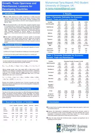
S1 Food, beverages and tobacco S5 Coke, petroleum products and nuclear fuel S2 Textiles, clothing and leather S6 Chemicals and chemical products Variables S1 S2 S3 S4 S5 S6 S7 S8 S3 Wood and wood products S7 Rubber and plastic products ln tariff -4.312 (0.00) -16.28 (0.00) -19.91 (0.00) -20.84 (0.00) -2.422 (0.38) -7.357 (0.06) -26.83 (0.00) -12.86 (0.00) S4 Publishing, printing and reproduction of recorded media S8 Non-metallic mineral products ln distance -0.792 (0.00) -0.761 (0.00) -0.929 (0.00) -0.889 (0.00) -1.093 (0.00) -0.845 (0.00) -0.862 (0.00) -0.878 (0.00) ln conflict 0.138 (0.39 0.384 (0.04 -0.361 (0.13 -0.806 (0.00) -0.177 (0.51) -0.126 (0.44) -0.183 (0.21) 0.098 (0.45) Bilateral measure of common language 0.736 (0.00) 0.881 (0.00) 0.558 (0.00) 1.079 (0.00) 0.468 (0.00) 0.317 (0.01) 0.658 (0.00) 0.672 (0.00) Common border dummy variable 0.509 (0.00) 0.217 (0.02) 0.526 (0.00) 0.681 (0.00) 0.865 (0.00) 0.174 (0.04) 0.586 (0.00) 0.733 (0.00) Bilateral measure of Southern hemisphere .. .. .. .. .. .. .. .. Pseudo R2 0.91 0.93 0.95 0.93 0.84 0.95 0.96 0.94 Regression results for some sectors Note: Pr>|z| in parenthesis; Number of observations for all sectors: 20356
- Within-sample predictions based on gravity estimations - Residuals in relative terms (varies between –100% and +100%) Trade potentials If 0%, predicted trade is close to current trade If > 30% untapped trade potential If < -30% strong current trade (above predicted). Bilateral FDI often explains those type of discrepancies - Alternative measure: use 95% prediction intervals
TradeSim should be seen as an interesting input and/or point of departure for asking the right questions and for stimulating in-depth analysis related to: trade policy issues and strategies (design, negociations) ex post. trade development programmes (South-South trade, export promotion)
Within sample predictions => Predictions depend on the sample choice (multilateral resistance term) Other possible determinants of trade flows, such as FDI, SPS/TBT, export subsidies and quantitative restrictions (quotas) are not taken into account Specialization patterns of small countries difficult to capture (mono-exporters) Some caveats
S1 Food, beverages and tobacco S5 Coke, petroleum products and nuclear fuel S2 Textiles, clothing and leather S6 Chemicals and chemical products Variables S1 S2 S3 S4 S5 S6 S7 S8 S3 Wood and wood products S7 Rubber and plastic products ln tariff -4.312 (0.00) -16.28 (0.00) -19.91 (0.00) -20.84 (0.00) -2.422 (0.38) -7.357 (0.06) -26.83 (0.00) -12.86 (0.00) S4 Publishing, printing and reproduction of recorded media S8 Non-metallic mineral products ln distance -0.792 (0.00) -0.761 (0.00) -0.929 (0.00) -0.889 (0.00) -1.093 (0.00) -0.845 (0.00) -0.862 (0.00) -0.878 (0.00) ln conflict 0.138 (0.39 0.384 (0.04 -0.361 (0.13 -0.806 (0.00) -0.177 (0.51) -0.126 (0.44) -0.183 (0.21) 0.098 (0.45) Bilateral measure of common language 0.736 (0.00) 0.881 (0.00) 0.558 (0.00) 1.079 (0.00) 0.468 (0.00) 0.317 (0.01) 0.658 (0.00) 0.672 (0.00) Common border dummy variable 0.509 (0.00) 0.217 (0.02) 0.526 (0.00) 0.681 (0.00) 0.865 (0.00) 0.174 (0.04) 0.586 (0.00) 0.733 (0.00) Bilateral measure of Southern hemisphere .. .. .. .. .. .. .. .. Pseudo R2 0.91 0.93 0.95 0.93 0.84 0.95 0.96 0.94 Annex 1: Regression results by sectorSecondary Sector (Tradesim, version 3) Note: Pr>|z| in parenthesis; Number of observations for all sectors: 20356
Excluding FDI Including FDI Importing country Current trade 2002-2003, US$ mio. TOTAL FDI stock 2003, US$ mio. Trade Potential, US$ mio. Relative residual Trade Potential, US$ mio. Relative residual Primary sector USA 414 2249 0.02 223 29.9 1023 -42.4 United Kingdom 1645 6639 0.37 135 84.8 1124 18.8 Mauritius 33 618 11.83 116 -54.9 342 -82.0 Mozambique 58 764 17.68 562 -81.4 1644 -93.2 Zimbabwe 87 306 1.72 291 -53.9 440 -66.9 Zambia 52 62 1.43 291 -69.6 186 -53.6 Secondary sector USA 3133 2249 0.02 187 88.7 924 54.5 United Kingdom 1734 6639 0.37 192 79.9 1385 11.2 Mauritius 232 618 11.83 135 26.4 374 -23.4 Mozambique 613 764 17.68 311 32.5 1163 -30.9 Zimbabwe 855 306 1.72 359 40.8 498 26.4 Zambia 511 62 1.43 289 27.7 185 46.7 Comparing trade potentials including FDI inthe Gravity Equation
Annex 2: deriving the gravity equation (Armington + CES): Consumers in region j maximize: (1) Subject to their budget constraint: (2) Consumption by region j consumers of goods from region i With: σ Elasticity of substitution between all goods Positive distribution parameter Nominal income of region j residents Price of region i goods for region j consumers
assuming and and Substituting in (1) and (2) and maximizing yields the nominal demand for region i goods by region j consumers: (3) With the consumer price index of region j (4)
The sum of i’s exports to all countries must equal i’s GDP (5) Substituting (5) into (3) (6) with defining (7)
Substituting (7) into (6) (8) And substituting (5) into (4) (9) Assuming symmetric trade barriers, i.e. , (7) and (9) can be solved, yielding (10) Yielding the Gravity Equation (11)