Download
1 / 29
320 likes | 836 Views
Flow Resistance, Channel Gradient, and Hydraulic Geometry. 1. Flow Resistance Uniformity and steadiness, turbulence, boundary layers, bed shear stress, velocity 2. Longitudinal Profiles Channel gradient, downstream fining 3. Hydraulic Geometry

E N D
Flow Resistance, Channel Gradient, and Hydraulic Geometry 1. Flow Resistance • Uniformity and steadiness, turbulence, boundary layers, bed shear stress, velocity 2. Longitudinal Profiles • Channel gradient, downstream fining 3. Hydraulic Geometry • General tendencies for exponents, technique for stream gaging
Flow Resistance Equations • Chezy (1769) • Manning (1889) • Darcy-Weisbach (SI units)
Resistance Coefficients • By assuming a roughness coefficient, u can be determined • Use an input parameters for numerical models (Julien, 2002)
Resistance Coefficients as a function of Bed Shear Stress (Bed Configuration) (van Rijn, 1993)
3. Longitudinal Profiles Outline • Controls on channel gradient • Downstream variations in discharge, bed slope, and bed texture (downstream fining) • Downstream fining channel concavity
Amazon River Longitudinal Bed Profile Rhine River (Knighton, 1998)
River Bollin Nigel Creek River Towy Longitudinal Bed Profile (Knighton, 1998)
Controls on Gradient (1) • Mackin (1948) - Concept of a graded stream: Over a period of time, slope is delicately adjusted to provide, with available discharge and channel characteristics, just the velocity required to transport the load supplied • Rubey (1952): for a constant w/d, S Qs, M (size of bed material load), 1/Q
Controls on Gradient (2) • Leopold and Maddock (1953): S 1/Q • Lane (1955): Expanded concept of graded stream • Hack (1957): S D50, 1/AD
Longitudinal Variations in Q, S, and Bed Texture, MS River +4° -3° -3°
Downstream Fining MS River Allt Dubhaig
Downstream Fining • D0 initial grain size, L downstream distance, a sorting or abrasion coefficient • Sternberg abrasion equation • Abrasion – mechanical breakdown of particles during transport; rates of DS fining >> rates of abrasion • Weathering – chemical and mechanical due to long periods of exposure; negligible • Hydraulic Sorting – size selective deposition • mainly due to a downstream decrease in bed shear stress and turbulence intensity of the river
For Mississippi River Data QB (cfs) SDB (mm) d (m) t (Pa) US 260 0.035 270 0.4 124 DS 2,070,000 0.00008 0.16 13 10 +4° -3° -3° +1° -1° d = cQf, f ~ 0.3 to 0.4 S = tQz, z ~ -0.65 t = gdS t ds, t (Qf)(Qz) t Qn, where n = -0.25 to -0.35 Assuming t0 ~ tcmax downstream fining
1D Exner Equation Change in bedload with distance with gain/loss to suspended load as modulated by grain settling velocity Change in bed height with time Change in total load with distance • Volume transport rates • Can be written for sediment mixtures and multiple dimensions • Spatial gradients in Qs due to spatial gradients in t • Slope adjustment, and downstream fining, can be brought on by aggradation and degradation
DS Fining Profile Concavity? • Modeling suggests the time-scale for sorting processes to produce downstream fining is shorter than the timescale for bed slope adjustment • Fluvial systems adjust their bed texture in response to spatial variations in shear stress and sediment supply
x Rod Level e1 Rod d1 e2 x1, y1 Water surface Ground surface d2 Water surface slope: (taken positive in the downstream direction) x = x2 x1 y = (e2d2) (e1d1) slope = y/x x2, y2 Measurement of Stream Channel Gradient Ground surface slope ≠ water surface slope
Hydraulic Geometry • Q is the dominant independent parameter, and that dependent parameters are related to Q via simple power functions • Applied “at-a-station” and “downstream”
DS Determining hydraulic geometry (Richards, 1982)
f = 0.52 At-a-station; Sugar Creek, MD m = 0.30 b = 0.18 (Leopold, Wolman, and Miller, 1964)
Downstream Same flow frequency (Morisawa, 1985)
m > f > b and m > b + f b = 0-0.2 f = 0.3-0.5 m = 0.3-0.5 At-a-station (Knighton, 1998)
Downstream b > f > m; b~0.5, f~0.4, m~0.1 (Knighton, 1998)
Hydraulic Geometry • At-a-station: rectangular channels; increase in discharge is “accommodated” by increasing flow depth and flow velocity • Downstream: increase in discharge is “accommodated” by increasing flow width and depth
Hydraulic Geometry as a Tool • Used in stream channel design • Identification of unstable stream corridors and unstable stream systems • Concept of channel equilibrium
Additional Considerations • Channel geometry also controlled by • Grain size and bed composition • Sediment transport rate (bed mobility and roughness) • Bank strength, as assessed by silt-clay content • Vegetation—different exponents depending upon presence and type • Curved channels and non-linear trends (compound channels) • Pools & riffles—different exponents
Additional Considerations depth velocity width (Richards, 1982)
Typical Stream Discharge Determination w0,d0,v0 wn+1,dn+1,vn+1 Tape measure w1 w2 wn,dn,vn w3 T T Q1 Q2 Q3 Qn Qn+1 Right Benchmark (looking downstream) Left Benchmark (looking downstream) d1 d2 d3 v1 Ground surface Current meter For d<0.75 m, located at 0.4d ; For d>0.75 m, average of 0.2d and 0.8d v2 v3 Discharge determination: Discharge = width depth velocity Q = w d v Q = Q1 + Q2 + Q3 … + Qn+1
Implications for Stream Restoration • Roughness coefficients (1) enable determination of velocity and (2) are critical input parameters for numerical models • Exner equation is most commonly used analytic expression to determine bed stability • Hydraulic geometry is (1) the most widely used analytic framework for stream channel design, and (2) used in the identification of unstable stream corridors and unstable stream systems
Conclusions • Flow velocity can be determined by assuming a friction coefficient • Downstream variations in channel gradient, bed texture, and bed shear stress despite increases in discharge and total sediment load • Hydraulic geometry assumes discharge is the primary independent parameter • Hydraulic geometry of river channels shows world-wide tendencies; very powerful “tool” • A technique for gaging streams is presented