Download
1 / 33
340 likes | 642 Views
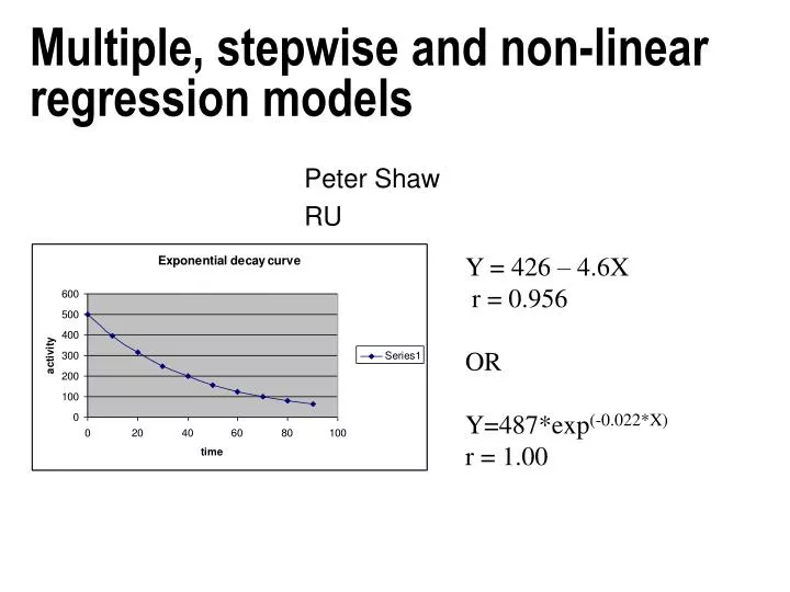
Multiple, stepwise and non-linear regression models. Peter Shaw RU. Y = 426 – 4.6X r = 0.956 OR Y=487*exp (-0.022*X) r = 1.00. Introduction. Last week we met and ran bivariate correlation/regression analyses, which were probably simple and familiar to most of you.

E N D
Multiple, stepwise and non-linear regression models Peter Shaw RU Y = 426 – 4.6X r = 0.956 OR Y=487*exp(-0.022*X) r = 1.00
Introduction Last week we met and ran bivariate correlation/regression analyses, which were probably simple and familiar to most of you. This week we extend this concept, looking at variants; MLR simple and stepwise, and non-linear regressions. The universals here are linear regression equations, and goodness of fit estimated as R2. The bivariate r we met last week is not meaningful in many cases here.
Multiple Linear Regression, MLR • MLR is just like bivariate regression, except that you have multiple independent (“explanatory”) variables. • Model: • Y = A + B*X1 + C*X2 (+ D*X3….) • Very often the explanatory variables are co-correlated, hence the dislike of the term “independents” • The goodness of fit is indicated by the R2 value, where R2 = proportion of total variance in Y which is explained by the regression. This is just like bivariate regression, except that we don’t used a signed (+/-) r value. • (Why no r? Because with 2 variables the line either goes up or down. With 3 variables the line can go +ve wrt X1 and -ve wrt X2)
A three dimensional data space. The 3-D graph of flower number, leaf length and plant height, seen from two rotations. Three variables define a three-dimensional data space, which can be visualised using three-dimensional graphs. No. flowers 60 Leaf 1, mm 30 50 Height 1st Leaf No.flowers mm mm 108 12 18 111 11 10 147 23 22 218 21 14 240 37 12 223 30 25 242 28 45 480 77 40 290 40 50 263 55 30 250 Height, mm 500 No. flowers 60 30 500 Height, mm 250 100 Leaf 1, mm
Figure 3.19. The 3-D graph relating crake density to mowing date and vegetation type. The width of the circles indicates corncrake number, ranging from 0 to the maximum of 10.
Erosion depth on marble tombstones in three Sheffield churchyards as a function of the age of the stone. Basic regression equation: Y = -0.03 + 0.027*X [Nb there’s an argument for forcing A = 0, but I’ll skip that] 3.0 2.0 Depth, mm 1.0 Rural site City edge 0 0 City centre 50 100 Age, years
Erosion depth on marble tombstones in three Sheffield churchyards as a function of the age of the stone. A separate regression line has been fitted for each of the three churchyards. erosion = 0.42 + 0.024*age + -0.13*distance, R2=0.73 (97 df) which can be compared with the bivariate equation: erosion = -0.28 + 0.027*age, R2 = 0.63 (98 df). 3.0 There are several philosophical catches here: Intercept? Parallel lines? Leads to ancova 2.0 Key Depth, mm 1.0 Rural site City edge 0 City centre 0 50 100 Age, years
Notice how adding a second explanatory variable increased the % variance explained – this is the whole point of MLR. In fact adding an explanatory variable is ALMOST CERTAIN to increase the R2 – if it does not, it must be perfectly correlated with the first explanatory variable (or have zero variance). The question is really whether it is worth adding that new variable? SRCE df SS MS F Age 1 58.995 3 58.995 167** Error 98 34.533 .352 Total 99 93.529 How does this relate to R2? Recall that R2 = % variance explained = 58.995/93.529 = 0.6308 SRCE df SS MS F A&D 2 68.33 34.166 131** Error 97 25.196 0.26 Total 99 93.529 H0: MS (A&D-A) = MS error F1,97 = (68.33-58.995)/1/0.26 = 35.9**
This leads to Stepwise MLR Given 1 dependent variable and lots of explanatory variables, start by finding the single highest correlation, and if significant, iterate: 1: Find the explanatory variable that causes the greatest reduction in error variance 2: Is this reduction significant? If so add to the model and repeat.
Data dredging tip: If you have (say) 50 spp, and want to find out quickly which one shows the sharpest response to a 1or0 factor (MF, logged vs unlogged etc), try this: Set the factor as dependent, then run stepwise MLR using all spp as predictors of that factor. Eccentric but works like a charm!
MLR is powerful and dangerous: MLR is widely used in research, especially for “data dredging”. • It gives accurate R2 values, and valid least-squares estimates of parameters – intercept, gradients wrt X1, X2 etc. • Sometimes its power can seem almost magical – I have a neat little dataset in which MLR can derive parameters of the polynomial function • xX = A + B*X + C*X2 + D*X3…
Empirically fitting polynomial functions by MLR: The triangular function We can find the general relation between number of points and number of rows – empirically! We solve the polynomial by MLR, then 1+2+3+4..+99+100 = ?
The case of the mysterious tipburn on the CEGB’s Scots Pine We had some homogenous aged pines exposed to SO2 in a sophisticated open-air fumigation system, max c. 200ppb. Books told us that Pine only got visible injury above 100 ppm – so we were well into the invisible damage region. Except that it wasn’t invisible on a few plants! About 5% were sensitive and could show damage in our conditions. Apart from DNA, what was going on? Tipburn on Pinus sylvestris in Liphook open air fumigation experiment 1985-1990 Data structure 35 rows of data = 7 plots * 5 years #plants burnt (=dep) then columns describing SO2. Column: annual mean; 12 * monthly mean; 52*weekly mean; 365 * daily mean, rather more hourly means .. Stepwise MLR picked up the mean SO2 conc. during the week of budburst as best predictor. Bingo!
But beware! • There is a serious pitfall when the explanatory variables are co-correlated (which is frequent, almost routine). • In this case the gradients should be more-or-less ignored! They may be accurate, but are utterly misleading. • An illustration: Y correlates +vely with X1 and with X2. • Enter Y, X1 and X2 into an MLR • Y = A + B*X1 + C*X2 • But if B >0, C may well be < 0! On the face of it this suggests that Y is –vely correlated with X2. • In fact this correlation is with the residual information content in X2 after its correlation with X1 is removed. • At least one multivariate package (CANOCO) instructs that prior to analysis you must ensure all explanatory variables are uncorrelated, by excluding offenders from the analysis. • This caveat is widely ignored, indeed widely unknown.
Colinearity & Variance inflation factors To diagnose colinearity, compute the VIF for each variable: VIFj = 1/(1-R2j) Where R2j is the multiple R2 between variable J and all others. If your maximum VIF > 10, worry! Exclude variables or run a PCA (coming up soon!)
Non-linear regressions • You should now be familiar with the notion of fitting a best fit line to a scattergraph, and the use of an R2 value to assess the significance of a relationship. • Be aware that linear regression implicitly fits a straight line - it would be possible to have a perfect relationship between dependent & independent variables, but r is non-significant! R = 0.95** R = 0 NS
Sometimes straight lines just aren’t enough! Are these data linear? X Y 0 0 1 1 2 4 3 9 4 16 5 25 6 36 R = 0.96 P<0.05 Y = 8X - 9.33 - but is it?!
There are many cases where the line you want to fit is not a straight one! • Population dynamics are often exponential (up or down), as are many physical processes such as heating/cooling, radioactive decay etc. • Body size relationships (allometry) are almost always curvy. • Almost always it is still possible to use familiar, unsophisticated linear regression on these. You just have to apply a simple mathematical trick first. Temp time BMR Mass
To illustrate the basic idea.. Take these clearly non-linear data. Y correlates well with X, but by calculating a new variable the correlation can be made perfect. X Y 0 0 1 1 2 4 3 9 4 16 5 25 6 36 Y# 0 1 2 3 4 5 6 Calculate Y# = Square root(Y) It is now evident that the correlation between X and Y* is perfect. Y# = 1*X + 0, r = 1.0, p<0.01
Logarithms.. • For better or worse, the tricks we need to straighten lines are based on the mathematical functions called logarithms. • When I were a lad… we used “logs” at school every day for long multiplications/divisions. Calculators stopped all that, and I find that I have to explain the basics here. • Forgive me if you already know this – someone sitting next to you won’t!
Let’s start with a few powers: • N 2N 3N 10N • 0 1 1 1 • 1 2 3 10 • 2 4 9 100 • 3 8 27 1000 • 4 16 81 10000 • 5 32 243 100000 • 6 64 729 1000000 • Given these we see that 26 64, 34 = 81 etc. • An alternative way of expressing this is to say that the Logarithm base 2(64) = 6, logarithm base 3(81) = 4. • This is abbreviated: • Log2(16) = 4, log3(9) = 2 etc.
In practice you are not offered log base 2 or 3 on calculators, though they are easy to work out. • What you do get is log10 or loge, where e = 2.7182818… Loge is usually written Ln. • The power of logs is that they translate multiplication into addition! • This is easy to see, sticking for a moment with logs base 2 • 8 * 4 = • (2 * 2 * 2) * (2 * 2) [23 * 22] • = (2*2*2*2*2) [25] • =32 [Note 3+2 =5] • Universally: Logx(A) + Logx(B) = Logx(A*B) • For virtually any values of x, A and B. (Exclude numbers <=0)
Which log to use? • Answer: It generally makes no difference at all! PROVIDING you are consistent. Throughout this lecture I will use ln = loge, but I could equally have used log10. • In case you wanted to know: • Loge(X) = log10(x) *loge(10) ETC • The case where you need to be careful is fitting an explicitly exponential model, but if you calculate a half life you will get the same answer in any log base.
Given this we can deal with 2 distinct types of non-linear relationship which cover >95% of biological/environmental situations. • 1: Exponential curves. These come out of population dynamics, where growth and decline typically involve proportionate changes (ie 10% per year) and have a doubling time or a half life. • Power relationships, where doubling the independent variable changes the dependent by 2X where X is the power constant. This gives us the allometric relationships typical of size scaling functions (body size/BMR, river diameter/discharge etc).
Exponential models B<0 = exponential decay This never quite goes flat but heads to an asymptote • The model can be recognised by having a half life or doubling time, and is defined as follows: • Y = A*exp(B*X) • Where A,B are constants, exp(x) is the natural antilog ex = 2.718x • Transform by getting log(Y) • Ln(y) = ln(A) + B*X B>0 = exponential growth. This is explosive – never persists long!
For exponential data: • Plot log(Y) vs X, and use regression to get the intercept + gradient. • Intercept = ln(A), gradient = B • If you want the half life, use: • T½ = ln(½)/B • Notice that the gradient will vary according to log base, so half life is safer as it doesn’t.
Count Time 500 0 400 10 320 20 240 30 200 40 160 50 120 60 100 70 85 80 70 90 A basic linear fit: Y = 426 – 4.6X r = 0.956
Log-transform the Y axis! Y = 6.19 – 0.022, r = 1 Hence Y=487*exp(-0.022*X) From this we get: Half life = ln(0.5)/-0.022 = 31.5sec
Power relationships(allometric models) • Here the model is: • Y = A*XB • A,B are constants as before • Linearise by log-transforming Y AND X • Ln(Y) = ln(A)+ln(X)*B • Plot ln(y) vs ln(X): intercept = ln(A), gradient = B BMR Mass
Y X LogY LogX logY = -0.155 + 0.5*log10X Hence Y = 0.7*sq. root(X)
To summarise: • 1: plot and inspect data • 2: explore by getting r value for • I: Y vs X [linear] • II: ln(Y) vs X [exponential] • III: ln(Y) vs ln(X) [allometric] • The best r value implies the best model, though the differences can be very minor.
This won’t always work! • Some models defy linear transformations. The commonest example is a quadratic relationship • Y = A + B*X + C*X2 Here there is no alternative but to call up a very powerful, general procedure, the general linear model (GLM). SPSS offers this as well as quadratic regression: you get an r value + estimates of A, B and C. Handle this just as we solved the triangular function above. N flux from soil Insect density