Primitive Recursive Functions (Chapter 3)

1. Primitive Recursive Functions(Chapter 3)

2. Preliminaries: partial and total functions • The domain of a partial function on set A contains the subset of A. • The domain of a total function on set A contains the entire set A. • A partial functionf is called partially computable if there is some program that computes it. Another term for such functions partial recursive. • Similarly, a function f is called computable if it is both total and partially computable. Another term for such function is recursive.

3. Composition • Let f : A → B and g : B → C • Composition of f and g can then be expressed as: g ͦ f : A → C (g ͦ f)(x) = g(f(x)) h(x) = g(f(x)) • NB: In general composition is not commutative: ( g ͦ f )(x) ≠ ( f ͦ g )(x)

4. Composition • Definition: Let g be a function containing k variables and f1 ... fk be functions of n variables, so the composition of g and f is defined as: • h(0) = k Base step h( x1, ... , xn) = g( f1(x1 ,..., xn), … , fk(x1 ,..., xn) ) Inductive step • Example: h(x , y) = g( f1(x , y), f2(x , y), f3(x , y) ) • h is obtained from g and f1... fk by composition. • If g and f1...fk are (partially) computable, then h is (partially) computable. (Proof by construction)

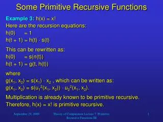
5. Recursion • From programming experience we know that recursion refers to a function calling upon itself within its own definition. • Definition: Let g be a function containing k variables then h is obtained through recursion as follows: h(x1 , … , xn) = g( … , h(x1 , … , xn) ) Example: x + y f( x , 0 ) = x(1) f(x , y+1 ) = f( x , y ) + 1(2) Input: f ( 3, 2 ) => f ( 3 , 1 ) + 1 => ( f ( 3 , 0 ) + 1 ) + 1 => ( 3 + 1 ) + 1 => 5

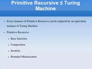
6. PRC: Initial functions • Primitive Recursively Closed (PRC) class of functions. • Initial functions: • Example of a projection function:u2 ( x1 , x2 , x3 , x4 , x5 ) = x2 • Definition: A class of total functions Cis called PRC² class if: • The initial functions belong to C. • Function obtained from functions belonging to C by either composition or recursion belongs to C. s(x) = x + 1 n(x) = 0 ui (x1 , … , xn) = xi

7. PRC: primitive recursive functions • There exists a class of computable functions that is a PRC class. • Definition: Function is considered primitive recursive if it can be obtained from initial functions and through finite number of composition and recursion steps. • Theorem: A function is primitive recursive iff it belongs to the PRC class. (see proof in chapter 3) • Corollary: Every primitive recursive function is computable.

8. Primitive recursive functions: sum • We have already seen the addition function, which can be rewritten in LRR as follows: sum( x, succ(y) ) => succ( sum( x , y)) ; sum( x , 0 ) => x ; Example:sum(succ(0),succ(succ(succ(0)))) => succ(sum(succ(0),succ(succ(0)))) => succ(succ(sum(succ(0),succ(0)))) => succ(succ(succ(sum(succ(0),0) => succ(succ(succ(succ(0))) => succ(succ(succ(1))) => succ(succ(2)) => succ(3) => 4 NB: To prove that a function is primitive recursive you need show that it can be obtained from the initial functions using only concatenation and recursion.

9. Primitive recursive functions: multiplication h( x , 0 ) = 0 h( x , y + 1) = h( x , y ) + x • In LRR this can be written as: mult(x,0) => 0 ; mult(x,succ(y)) => sum(mult(x,y),x) ; • What would happen on the following input? mult(succ(succ(0)),succ(succ(0)))

10. Primitive recursive functions: factorial 0! = 1 ( x + 1 ) ! = x ! * s( x ) • LRR implementation would be as follows: fact(0) => succ(null(0)) ; fact(succ(x)) => mult(fact(x),succ(x)) ; Output for the following? fact(succ(succ(null(0))))

11. Primitive recursive functions: power and predecessor Power function In LRR the power function can be expressed as follows: pow(x,0) => succ(null(0)) ; pow(x,succ(y)) => mult(pow(x,y),x) ; Predecessor function In LRR the predecessor is as follows: pred(1) => 0 ; pred(succ(x)) => x ; p (0) = 0 p ( t + 1 ) = t

12. Primitive recursive functions: ∸, | x – y | and α dotsub(x,x) => 0 ; dotsub(x,succ(y)) => pred(dotsub(x,y)) ; x ∸ 0 = x x ∸ ( t + 1) = p( x ∸ t ) What would be the output? • dotsub(succ(succ(succ(0))),succ(0)) | x – y | = ( x ∸ y ) + ( y ∸ x ) abs(x,y) => sum(dotsub(x,y),dotsub(y,x)) ; α(x) = 1 ∸ x α(x) => dotsub(1,x) ; Output for the following? • a(succ(succ(0))) • a(null(0))

13. Primitive recursive functions

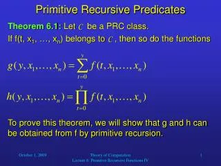
14. Bounded quantifiers • Theorem: Let C be a PRC class. If f( t , x1 , … , xn) belongs to C then so do the functions g( y , x1 , ... , xn ) = f( t , x1 , …, xn ) g( y , x1 , ... , xn ) = f( t , x1 , …, xn )

15. Bounded quantifiers • Theorem: Let C be a PRC class. If f( t , x1 , … , xn) belongs to C then so do the functions g( y , x1 , ... , xn ) = f( t , x1 , …, xn ) g( y , x1 , ... , xn ) = f( t , x1 , …, xn ) • Theorem: If the predicate P( t, x1 , … , xn ) belongs to some PRC class C, then so do the predicates: ( t)≤y P(t, x1, … , xn ) (∃t)≤y P(t, x1, … , xn )

16. Primitive recursive predicates Exercises for Chapter 3: page 62 Questions 3,4 and 5. Fibonacci function

17. Bounded minimalization Let P(t, x1, … ,xn) be in some PRC class C and we can define a function g as follows:

18. Bounded minimalization Let P(t, x1, … ,xn) be in some PRC class C and we can define a function g as follows: ,where

19. Bounded minimalization Let P(t, x1, … ,xn) be in some PRC class C and we can define a function g as follows: ,where • Function g also belongs to C as it is attained from composition of primitive recursive functions.

20. Bounded minimalization Let P(t, x1, … ,xn) be in some PRC class C and we can define a function g as follows: ,where • Function g also belongs to C as it is attained from composition of primitive recursive functions. • t0 is the least value for for which the predicate P is true (1).

21. Bounded minimalization Let P(t, x1, … ,xn) be in some PRC class C and we can define a function g as follows: ,where • Function g also belongs to C as it is attained from composition of primitive recursive functions. • t0 is the least value for for which the predicate P is true (1).

22. Bounded minimalization Let P(t, x1, … ,xn) be in some PRC class C and we can define a function g as follows: ,where • Function g also belongs to C as it is attained from composition of primitive recursive functions. • t0 is the least value for for which the predicate P is true (1).

23. Bounded minimalization Let P(t, x1, … ,xn) be in some PRC class C and we can define a function g as follows: ,where • Function g also belongs to C as it is attained from composition of primitive recursive functions. • t0 is the least value for for which the predicate P is true (1).

24. Bounded minimalization Let P(t, x1, … ,xn) be in some PRC class C and we can define a function g as follows: ,where • Function g also belongs to C as it is attained from composition of primitive recursive functions. • t0 is the least value for for which the predicate P is true (1). • g( y , x1 , ... , xn ) produces the least value for which P is true. Finally the definition for bounded minimalization can be given as:

25. Bounded minimalization Let P(t, x1, … ,xn) be in some PRC class C and we can define a function g as follows: ,where • Function g also belongs to C as it is attained from composition of primitive recursive functions. • t0 is the least value for for which the predicate P is true (1). • g( y , x1 , ... , xn ) produces the least value for which P is true. Finally the definition for bounded minimalization can be given as: • Theorem: If P(t,x1, … ,xn) belongs to some PRC class C and there is function g that does the bounded minimalization for P, then f belongs to C.

26. Unbounded minimalization • Definition: y is the least value for which predicate P is true if it exists. If there is no value of y for which P is true, the unbounded minimalization is undefined.

27. Unbounded minimalization • Definition: y is the least value for which predicate P is true if it exists. If there is no value of y for which P is true, the unbounded minimalization is undefined. • We can then define this as a non-total function in the following way:

28. Unbounded minimalization • Definition: y is the least value for which predicate P is true if it exists. If there is no value of y for which P is true, the unbounded minimalization is undefined. • We can then define this as a non-total function in the following way: • Theorem: If P(x1, … , xn, y) is a computable predicate and if then g is a partially computable function. (Proof by construction)

29. Additional primitive recursive functions • [ x / y ] , the whole part of the division i.e. [10/4]=2 • R(x,y) , remainder of the division of x by y. • pn , nth prime number i.e p1=2 , p2=3 etc.

30. Pairing functions • Let us consider the following primitive recursive function that provides a coding for two numbers x and y.

31. Pairing functions • Let us consider the following primitive recursive function that provides a coding for two numbers x and y. Example: <1,1> = 2 * ( 2 + 1 ) ∸ 1 = 6 ∸ 1 = 5 <1,2> = 2 * ( 2*2 + 1) ∸ 1 = 10 ∸ 1 = 9

32. Pairing functions • Let us consider the following primitive recursive function that provides a coding for two numbers x and y. Example: <1,1> = 2 * ( 2 + 1 ) ∸ 1 = 6 ∸ 1 = 5 <1,2> = 2 * ( 2*2 + 1) ∸ 1 = 10 ∸ 1 = 9

33. Pairing functions • Let us consider the following primitive recursive function that provides a coding for two numbers x and y. Example: <1,1> = 2 * ( 2 + 1 ) ∸ 1 = 6 ∸ 1 = 5 <1,2> = 2 * ( 2*2 + 1) ∸ 1 = 10 ∸ 1 = 9 • Define z to be as: < x , y > = z Then for any z there is always a unique solution x and y.

34. Pairing functions • Let us consider the following primitive recursive function that provides a coding for two numbers x and y. Example: <1,1> = 2 * ( 2 + 1 ) ∸ 1 = 6 ∸ 1 = 5 <1,2> = 2 * ( 2*2 + 1) ∸ 1 = 10 ∸ 1 = 9 • Define z to be as: < x , y > = z Then for any z there is always a unique solution x and y.

35. Pairing functions • Let us consider the following primitive recursive function that provides a coding for two numbers x and y. Example: <1,1> = 2 * ( 2 + 1 ) ∸ 1 = 6 ∸ 1 = 5 <1,2> = 2 * ( 2*2 + 1) ∸ 1 = 10 ∸ 1 = 9 • Define z to be as: < x , y > = z Then for any z there is always a unique solution x and y. • Thus we have the solutions for x and y which can then be defined using the following functions:

36. Pairing functions • More formally this can written as: • Pairing Function Theorem: functions <x,y>, l(z), r(z) have the following properties: • are primitive recursive • l(<x,y>) = x and r(<x,y>) = y • < l(z) , r(z) > = z • l(z) , r(z)≤ z

37. Gödel numbers • Let (a1, … , an) be any sequence, then the Gödel number is computed as follows:

38. Gödel numbers • Let (a1, … , an) be any sequence, then the Gödel number is computed as follows: • Example: Take a sequence (1,2,3,4), the Gödel number will be computed as follows:

39. Gödel numbers • Let (a1, … , an) be any sequence, then the Gödel number is computed as follows: • Example: Take a sequence (1,2,3,4), the Gödel number will be computed as follows: • Gödel numbering has a special uniqueness property: If [a1, … , an ] = [ b1, … , bn ] then ai = bi , where i = 1, … , n

40. Gödel numbers • Let (a1, … , an) be any sequence, then the Gödel number is computed as follows: • Example: Take a sequence (1,2,3,4), the Gödel number will be computed as follows: • Gödel numbering has a special uniqueness property: If [a1, … , an ] = [ b1, … , bn ] then ai = bi , where i = 1, … , n • Also notice: [ a1, … , an ] = [ a1, … , an, 0 ]

41. Gödel numbers • Given that x = [a1, … , an ], we can now define two important functions:

42. Gödel numbers • Given that x = [a1, … , an ], we can now define two important functions: • Example: Let x = [ 4 , 3 , 2 , 1 ], then (x)2 = 3 and (x)4=1 and (x)0 = 0

43. Gödel numbers • Given that x = [a1, … , an ], we can now define two important functions: • Example: Let x = [ 4 , 3 , 2 , 1 ], then (x)2 = 3 and (x)4=1 and (x)0 = 0 Lt(10) = will be the length of the sequence derived using Gödel numbering

44. Gödel numbers • Given that x = [a1, … , an ], we can now define two important functions: • Example: Let x = [ 4 , 3 , 2 , 1 ], then (x)2 = 3 and (x)4=1 and (x)0 = 0 Lt(10) = will be the length of the sequence derived using Gödel numbering So: 10 = 2^1 * 3^0 * 5^1 = [ 1, 0, 1 ] => Lt(10) = 3

45. Gödel numbers • Given that x = [a1, … , an ], we can now define two important functions: • Example: Let x = [ 4 , 3 , 2 , 1 ], then (x)2 = 3 and (x)4=1 and (x)0 = 0 Lt(10) = will be the length of the sequence derived using Gödel numbering So: 10 = 2^1 * 3^0 * 5^1 = [ 1, 0, 1 ] => Lt(10) = 3 • Sequence Number Theorem: (1)

46. Gödel numbers • Given that x = [a1, … , an ], we can now define two important functions: • Example: Let x = [ 4 , 3 , 2 , 1 ], then (x)2 = 3 and (x)4=1 and (x)0 = 0 Lt(10) = will be the length of the sequence derived using Gödel numbering So: 10 = 2^1 * 3^0 * 5^1 = [ 1, 0, 1 ] => Lt(10) = 3 • Sequence Number Theorem: (1) (2)