Recursion: Recursive Algorithms Explained
A detailed explanation of recursion in programming, including examples like factorial calculation, iterative vs. recursive implementation, and conditions for valid recursion. Learn how recursive functions work and when to use recursion effectively.

Recursion: Recursive Algorithms Explained
E N D
Presentation Transcript
Chapter 3: Recursive Algorithms 3.5 Recursion
What is recursion? • Sometimes, the best way to solve a problem is by solving a smaller version of the exact same problem first • Recursion is a technique that solves a problem by solving a smaller problem of the same type
When you turn this into a program, you end up with functions that call themselves (recursive functions) int f(int x) { int y; if(x==0) return 1; else { y = 2 * f(x-1); return y; } } What does this program does?
Problems defined recursively • There are many problems whose solution can be defined recursively • Example: n factorial 1if n = 0 n!=(closed form solution) 1*2*3*…*(n-1)*n if n > 0 1 if n = 0 n!= (recursive solution) (n-1)!*n if n > 0
Coding the factorial function • Iterative implementation int Factorial(int n) { int fact = 1; for(int count = 2; count <= n; count++) fact = fact * count; return fact; }
Coding the factorial function • Recursive implementation int Factorial(int n) { if (n==0) // base case return 1; else return n * Factorial(n-1); }
Recursion • Recursive methods • Methods that call themselves • Directly • Indirectly • Call others methods which call it • Continually breaks problem down to simpler forms • Divides the problem into two pieces: • a piece the method knows how to perform (base case) • a piece the method does no know how to perform
return 4 * 6 = 24 4! Final answer call recursiveFactorial(4) return 3 * 2 =6 call recursiveFactorial(3) return 2 * 1 =2 call recursiveFactorial(2) return 1 * =1 1 call recursiveFactorial(1) return 1 call recursiveFactorial(0)
Conditions for Valid Recursion • For recursive functions to work, the following two conditions must be met: • There must be a basis step ( base case) where the input value or size is • the smallest possible, and • in which case the processing is non-recursive. • The input (parameters) of every recursive call must be smaller in value or size than the input of the original function
Illustration of the Conditions long factorial(int n){ if (n==0) return 1; // basis step. Input value n is minimum (0). long m=factorial(n-1); // recursion. Input value of recursive call is n-1<n m *=n; return m; }
Recursion vs. iteration • Iteration can be used in place of recursion and vice versa • An iterative algorithm uses a looping construct • A recursive algorithm uses a branching structure • Recursion can simplify the solution of a problem, often resulting in shorter, more easily understood source code • Recursive solutions are often less efficient, in terms of both time and space, than iterative solutions
How is recursion implemented? • What happens when a function gets called? int a(int w) { return w+w; } int b(int x) { int z,y; ……………… // other statements z = a(x) + y; return z; }
What happens when a function is called? (cont.) An activationrecord is stored into a stack (run-time stack) • The computer has to stop executing function b and starts executing functiona • Since it needs to come back to functionblater, it needs to store everything about functionb that is going to need (x, y, z, and the place to start executing upon return) • Then,w of a is bounded tox from b • Control is transferred to functiona
What happens when a function is called? (cont.) • After function a is executed, the activation record is popped out of the run-time stack • All the old values of the parameters and variables in functionb are restored and the return value of functiona replaces a(x) in the assignment statement
What happens when a recursive function is called? • Except the fact that the calling and called functions have the same name, there is really no difference between recursive and nonrecursive calls int f(int x) { int y; if(x==0) return 1; else { y = 2 * f(x-1); return y+1; } }
2*f(2) int f(int x) { int y; if(x==0) return 1; else { y = 2 * f(x-1); return y+1; } } 2*f(1) 2*f(0) =f(0) =f(1) =f(2) =f(3)
Recursion can (sometimes) be very inefficient: Deciding whether to use a recursive solution • When the depthof recursive calls is relatively "shallow" • The recursive version is shorter and simpler than the nonrecursive solution • The recursive version does about the same amount of work as the nonrecursive version
How do I write a recursive function? • Determine the size factor • Determine the base case(s) (the one for which you know the answer) • Determine the general case(s) (the one where the problem is expressed as a smaller version of itself) • Verify the algorithm (use the "Three-Question-Method")
Three-Question Verification Method • The Base-Case Question: Is there a nonrecursive way out of the function, and does the routine works correctly for this "base" case? • The Smaller-Caller Question: Does each recursive call to the function involve a smaller case of the original problem, leading inescapably to the base case? • The General-Case Question: Assuming that the recursive call(s) work correctly, does the whole function work correctly?
Example of Recursion Example 3.1:Modern operating systems define file-system directories (which are also sometimes called "folders") in a recursive way. Namely, a file system consists of a top-level directory, and the contents of this directory consists of files and other directories, which in turn can contain files and other directories, and so on. The base directories in the file system contain only files, but by using this recursive definition, the operating system allows for directories to be nested arbitrarily deep. Example 3.2: An argument list in Java using the following notation: argument-list: argument argument-list, argument In other words, an argument list consists of either (i) an argument or (ii) an argument list followed by a comma and an argument.
Linear Recursion The simplest form of recursion is linear recursion, where a method is defined so that it makes at most one recursive call each time it is invoked. This type of recursion is useful when we view an algorithmic problem in terms of a first or last element plus a remaining set that has the same structure as the original set.
Summing the Elements of an Array Recursively We can solve this summation problem using linear recursion by observing that the sum of all n integers in A is • Equal to A[0], if n = 1, or • The sum of the first n − 1 integers in A plus the last element in A
Analyzing Recursive Algorithms using Recursion Traces Figure 3.24: Recursion trace for an execution of LinearSum(A,n) with input parameters A = {4,3,6,2,5} and n = 5.
Reversing an Array by Recursion • The problem of reversing the n elements of an array, A, so that the first element becomes the last, the second element becomes second to the last, and so on. • We can solve this problem using linear recursion, by observing that the reversal of an array can be achieved by swapping the first and last elements and then recursively reversing the remaining elements in the array.
Reversing an Array by Recursion • Code Fragment 3.32: Reversing the elements of an array using linear recursion.
Tail Recursion • Using recursion can often be a useful tool for designing algorithms that have elegant, short definitions. • When we use a recursive algorithm to solve a problem, we have to use some of the memory locations in our computer to keep track of the state of each active recursive call. • We can use the stack data structure, to convert a recursive algorithm into a nonrecursive algorithm, but there are some instances when we can do this conversion more easily and efficiently. Specifically, we can easily convert algorithms that use tail recursion. • An algorithm uses tail recursion if it uses linear recursion and the algorithm makes a recursive call as its very last operation. • For example, the algorithm of Code Fragment 3.31 does not use tail recursion, even though its last statement includes a recursive call. This recursive call is not actually the last thing the method does. After it receives the value returned from the recursive call, it adds this value to A [n − 1] and returns this sum. That is, the last thing this algorithm does is an add, not a recursive call. • When an algorithm uses tail recursion, we can convert the recursive algorithm into a nonrecursive one, by iterating through the recursive calls rather than calling them explicitly.
Tail Recursion Code Fragment 3.33: Reversing the elements of an array using iteration.
Binary Recursion • When an algorithm makes two recursive calls, we say that it uses binary recursion. • These calls can, for example, be used to solve two similar halves of some problem • As another application of binary recursion, let us revisit the problem of summing the n elements of an integer array A. • In this case, we can sum the elements in A by: (i) recursively summing the elements in the first half of A; (ii) recursively summing the elements in the second half of A; (iii) adding these two values together.
Binary Recursion • Code Fragment 3.34: Summing the elements in an array using binary recursion.
Binary Recursion • To analyze Algorithm BinarySum, we consider, for simplicity, the case where n is a power of two. • Figure 3.25 shows the recursion trace of an execution of method BinarySum(0,8). • We label each box with the values of parameters i and n, which represent the starting index and length of the sequence of elements to be reversed. • Notice that the arrows in the trace go from a box labeled (i,n) to another box labeled (i,n/2) or (i + n/2,n/2). That is, the value of parameter n is halved at each recursive.
Binary Recursion • The depth of the recursion, that is, the maximum number of method instances that are active at the same time, is 1 + log2n. • Thus, Algorithm BinarySum uses an amount of additional space roughly proportional to this value. This is a big improvement over the space needed by the LinearSum method of Code Fragment 3.31. • The running time of Algorithm BinarySum is still roughly proportional to n, however, since each box is visited in constant time when stepping through our algorithm and there are 2n − 1 boxes.
Merge-Sort • Merge-sort, can be described in a simple and compact way using recursion. Divide-and-Conquer • Merge-sort is based on an algorithmic design pattern called divide-and-conquer. • The divide-and-conquer pattern consists of the following three steps: 1. Divide: If the input size is smaller than a certain threshold (say, one or two elements), solve the problem directly using a straightforward method and return the solution so obtained. Otherwise, divide the input data into two or more disjoint subsets. 2. Recur: Recursively solve the subproblems associated with the subsets. 3. Conquer: Take the solutions to the subproblems and "merge" them into a solution to the original problem.
Merge Merge Sort: Idea Divide into two halves A FirstPart SecondPart Recursively sort SecondPart FirstPart A is sorted!
Merge-Sort: Merge Sorted A: merge Sorted SecondPart SortedFirstPart A: A[right] A[left] A[middle]
5 15 28 30 6 10 14 5 2 3 7 8 1 4 5 6 R: L: 3 5 15 28 6 10 14 22 Temporary Arrays Merge-Sort: Merge Example A:
Merge-Sort: Merge Example A: 3 1 5 15 28 30 6 10 14 k=0 R: L: 3 2 15 3 7 28 30 8 6 1 10 4 5 14 22 6 i=0 j=0
Merge-Sort: Merge Example A: 2 1 5 15 28 30 6 10 14 k=1 R: L: 2 3 5 3 15 7 8 28 6 1 10 4 14 5 6 22 i=0 j=1
Merge-Sort: Merge Example A: 3 1 2 15 28 30 6 10 14 k=2 R: L: 2 3 7 8 6 1 10 4 5 14 22 6 i=1 j=1
Merge-Sort: Merge Example A: 1 2 3 6 10 14 4 k=3 R: L: 2 3 7 8 1 6 10 4 14 5 6 22 j=1 i=2
Merge-Sort: Merge Example A: 1 2 3 4 6 10 14 5 k=4 R: L: 2 3 7 8 1 6 10 4 14 5 6 22 i=2 j=2
Merge-Sort: Merge Example A: 6 1 2 3 4 5 6 10 14 k=5 R: L: 2 3 7 8 6 1 4 10 5 14 6 22 i=2 j=3
Merge-Sort: Merge Example A: 7 1 2 3 4 5 6 14 k=6 R: L: 2 3 7 8 1 6 10 4 14 5 22 6 i=2 j=4
Merge-Sort: Merge Example A: 8 1 2 3 4 5 6 7 14 k=7 R: L: 2 3 5 3 7 15 28 8 6 1 10 4 5 14 22 6 i=3 j=4
Merge-Sort: Merge Example A: 1 2 3 4 5 6 7 8 k=8 R: L: 3 2 3 5 15 7 8 28 1 6 10 4 14 5 22 6 j=4 i=4
Divide and Conquer Examples • Binary search • Quicksort • Merge Sort • Tree traversals
Merge-Sort Using Divide-and-Conquer for Sorting • Recall that in a sorting problem we are given a sequence of n objects, stored in a linked list or an array, together with some comparator defining a total order on these objects, and we are asked to produce an ordered representation of these objects. • To allow for sorting of either representation, we will describe our sorting algorithm at a high level for sequences and explain the details needed to implement it for linked lists and arrays. • To sort a sequence S with n elements using the three divide-and-conquer steps, the merge-sort algorithm proceeds as follows:
Merge-Sort • Divide: • If S has zero or one element, return S immediately; it is already sorted. • Otherwise (S has at least two elements), remove all the elements from S and put them into two sequences, S1 and S2, each containing about half of the elements of S; • that is, S1 contains the first ⌈n/2⌉ elements of S, • and S2 contains the remaining ⌊n/2⌋ elements. 2. Recur: Recursively sort sequences S1 and S2. 3. Conquer: Put back the elements into S by merging the sorted sequences S1 and S2 into a sorted sequence.
Merge-Sort • Merge-sort on an input sequence S with n elements consists of three steps: • Divide: partition S into two sequences S1and S2 of about n/2 elements each • Recur: recursively sort S1and S2 • Conquer: merge S1and S2 into a unique sorted sequence AlgorithmmergeSort(S, C) Inputsequence S with n elements, comparator C Outputsequence S sorted • according to C ifS.size() > 1 (S1, S2)partition(S, n/2) mergeSort(S1, C) mergeSort(S2, C) Smerge(S1, S2)
Merge-Sort Tree • An execution of merge-sort is depicted by a binary tree • each node represents a recursive call of merge-sort and stores • unsorted sequence before the execution and its partition • sorted sequence at the end of the execution • the root is the initial call • the leaves are calls on subsequences of size 0 or 1 7 2 9 4 2 4 7 9 7 2 2 7 9 4 4 9 7 7 2 2 9 9 4 4
7 2 9 4 2 4 7 9 3 8 6 1 1 3 8 6 7 2 2 7 9 4 4 9 3 8 3 8 6 1 1 6 7 7 2 2 9 9 4 4 3 3 8 8 6 6 1 1 Execution Example • Partition 7 2 9 4 3 8 6 11 2 3 4 6 7 8 9