Download
1 / 30
330 likes | 616 Views
Networks in Metabolism and Signaling Edda Klipp Humboldt University Berlin Lecture 2 / WS 2007/08 Basic Principles of Graph Theory and Random Networks. Basic Principles of Graph Theory. Literature: J. Sedlácek (1968) Einführung in die Graphentheorie. Teubner Verlagsgesellschaft, Leipzig.

E N D
Networks in Metabolism and Signaling Edda Klipp Humboldt University BerlinLecture 2 / WS 2007/08Basic Principles of Graph Theory and Random Networks
Basic Principles of Graph Theory Literature: J. Sedlácek (1968) Einführung in die Graphentheorie. Teubner Verlagsgesellschaft, Leipzig. Albert & Barabási (2002) Statistical mechanics of complex networks. Rev Mod Physics, 74, 47-97. Barabási & Oltvai (2004) Network biology: understanding the cell’s functional organization, Nature Review Genetics, 5, 101-113.
Classical Examples The problem of “Fährmann, Ziege, Wolf und Heu” (W) (F,Z,W) (F,Z) (F,W,H) (F,Z,W,H) (Z) (0) (W,H) (H) (F,Z,H)
The Bridges of Königsberg Die Brücken von Königsberg Im Zentrum der preussischen Stadt Königsberg (heute Kaliningrad) bildet der Fluss Pregel beim Zusammenfluss zweier Arme eine Insel. Im 18. Jahrhundert verbinden 7 Brücken die Flussufer mit der Insel. Es stellt sich die Frage, ob es einen Rundweg gibt, bei dem man alle 7 Brücken genau einmal überquert und wieder zum Ausgangspunkt zurück gelangt. Geschichte Das Problem der Königsberger Brücken stammt von Leonhard Euler. Im Jahre 1736 beweist er, dass es keinen solchen Rundweg geben kann. Er betrachtet den allgemeinen Fall mit einer beliebigen Anzahl Inseln und Brücken und zeigt, dass ein Rundweg der gesuchten Art genau dann möglich ist, wenn sich an keinem der Ufer eine ungerade Zahl von Brücken befindet. Gibt es an genau zwei Ufern eine ungerade Anzahl Brücken, dann existiert ein Weg, der bei diesen beiden Ufern beginnt und endet und dabei alle Brücken genau einmal überquert. Gibt es, wie in Königsberg, mehr als zwei Gebiete, zu denen eine ungerade Zahl von Brücken führt, dann kann kein Weg existieren, der genau einmal alle Brücken überquert.
Graphs: Definitions vertex – Knoten edge – Kante tuple – Tupel, geordnete Menge set – Menge B vertex, node edge A C A graph is a tuple (V,E) with V a set of n vertices and a set of m edges E: G=(V,E) Example: Proteins – vertices, interactions – edges
Graphs: Completeness B Edge AB is has vertices A and B. Knoten A ist inzidiert mit Kante AB. vertex edge A C Be E0the set of all sub-sets of V with two elements. A graph is complete, if E=E0. d) a) b) c) G1=(V1,E1) G2=(V2,E2) If and : G1 and G2 are complementary. d)
Graph Types Undirected graphs: A B Directed graphs (digraphs): directed edge (i,j) E with idenoting the head and j denoting the tail of the edge. A A B B Extension: Directed edge (i,j,s)E with s{+1,-1} to represent activatory or inhibitory influences.
Graph Types: Biparite Graphs A C R1 B D Set of graph vertices decomposed into two disjoint sets such that no two graph vertices within the same set are adjacent. Graphs must represent two distinct classes of nodes such as metabolites (blue, circles) and reactions (yellow, boxes) ATP ADP R1 Fruc-6-P Fruc-1,6-P2
Graph Representation: Adjacency Matrix Adjacency matrix – Inzidenzmatrix A B E D C G F • Adjacency matrix A: non-zero entries represent edges - quadratic - unique assignment of adjacency matrix to graph - unique assignment of graph to adjacency matrix • Bipartite graphs: sub-matrices for the two classes of nodes • Alternative formats: edge lists, vertex lists
Graph Theoretical Measures: Degree Degree – Knotengrad A B E D C G F • Number of edges to which a vertex is connected: Degreek. • For directed graphs: in-degree – edges ending at a vertex out-degree – edges starting a vertex • Vertices with degree 0: isolated Be G a finite graph, v the number of nodes, k the number of edges and s1, s2,…su the degrees of the individual nodes, then holds:
Graph Theoretical Measures: Degree P(kin) 1/7 4/7 2/7 kin 0 1 2 A B E D C G F P(kout) 1/7 4/7 2/7 kout 0 1 2 • Global connectivity properties of a graph: Average degree <k> Degree distribution P(k) <kin> = (4x1 + 2x2)/7=8/7≈1,14 Degree distributions allow to distinguish between different types of networks
Einschub: Diskrete Wahrscheinlichkeitsverteilungen Binomialverteilung: p=1/2 P(k) Eigenschaften einer Stichprobe: Wenn das gewünschte Ergebnis eines Versuches die Wahrscheinlichkeit p besitzt, und die Zahl der Versuche n ist, dann gibt die Binomialverteilung an, mit welcher Wahrscheinlichkeit sich insgesamt k Erfolge einstellen. P(k) ist die Wahrscheinlichkeit (z.B. mit n Versuchen aus einem Topf von Bällen k schwarze zu ziehen) Summe aller Wahrscheinlichkeiten Erwartungswert (vgl.: Mittelwert für sehr viele Wiederholungen) E(X) = np Varianz Var(X) = np(1-p)
Einschub: Diskrete Wahrscheinlichkeitsverteilungen Poissonverteilung: Eigenschaften einer Stichprobe: Wie vorher, nur bei sehr kleiner Wahrscheinlichkeit der Einzelereignisse, z.B. weil n sehr groß. l - Ereignisrate (z.B. Fehlerrate bei der DNS-Replikation) Erwartungswert (vgl.: Mittelwert für sehr viele Wiederholungen) E(X) = l Var(X) = l Varianz 0.8 Exponentialverteilung: 0.6 0.4 E(X) = 1/l 0.2 Var(X) = 1/l2 0.0 0 20 40 60 80 100
Degree Distributions • Degree distribution of the World Wide Web from two different measurements: h, the 325 729-node sample of Albert et al. (1999); s, the measurements of over 200 million pages by Broder et al. (2000); • degree distribution of the outgoing edges; • degree distribution of the incoming edges. The data have been binned logarithmically to reduce noise. Albert & Barabasi, 2002, Rev Mod Phys
Degree Distributions The degree distribution of several real networks: (a) Internet at the router level. Data courtesy of Ramesh Govindan; (b) movie actor collaboration network. After Barabasi and Albert 1999. Note that if TV series are included as well, which aggregate a large number of actors, an exponential cutoff emerges for large k (Amaral et al., 2000); (c) co-authorship network of high-energy physicists. After Newman (2001a,2001b); (d) co-authorship network of neuroscientists. After Barabasi et al. (2001). Albert & Barabasi, 2002, Rev Mod Phys
Degree Distributions Connectivity distributions P(k) for substrates. a, Archaeoglobus fulgidus (archae); b, E. coli (bacterium); c, Caenorhabditis elegans (eukaryote), shown on a log±log plot, counting separately the incoming (In) and outgoing links (Out) for each substrate. kin (kout) corresponds to the number of reactions in which a substrate participates as a product (educt). d, The connectivity distribution averaged over all 43 organisms. Jeong H et al, 2000, Nature
Random Graphs First well-know example: Model of Paul Erdős and Alfréd Rényi History: Erdős number beschreibt die Distanz im Graphen der Koautorenschaft bezogen auf den Mathematiker Paul Erdős. Im Graphen werden die publizistisch verwandten Autoren als Knoten repräsentiert, zwischen denen jeweils dann eine Kante existiert, wenn sie eine Publikation gemeinsam verfasst haben. Paul Erdős selbst hat die Erdős-Zahl 0, alle Koautoren, mit welchen er publiziert hat, haben die Erdős-Zahl 1. Autoren, die mit Koautoren von Paul Erdős publiziert haben, haben die Erdős-Zahl 2 usw. Wenn keine Verbindung in dieser Form zu einer Person herstellbar ist, ist ihre Erdős-Zahl ∞. Es zeigt sich, dass die Erdős-Zahl der meisten Personen entweder unendlich oder erstaunlich gering ist. Letzteres rührt vor allem daher, dass Erdős mit über 500 verschiedenen Wissenschaftlern gemeinsam publizierte und er in vielen Teilbereichen der Mathematik bewandert war.
Random Graphs A well-know example: Model of Paul Erdős and Alfréd Rényi Start with N nodes. Connect every pair of nodes with probability p • Obtain graph with approx. ½ pN (N-1) edges Degree distribution: Poisson distribution Average degree: <k> = ½ pN (N-1) * 2/N = p(N-1) pN Dice number z [0;1]. If z<p then connection
Random Graphs: Evolution Construction of random graphs is called evolution. Starting with a set of Nisolated vertices, the graph develops by the successive addition of random edges. The graphs obtained at different stages of this process correspond to larger and larger connection probabilities p, eventually obtaining a fully connected graph having the maximum number of edges n=N(N-1)/2 for p1.
Random Networks Questions: Are real networks really random? Display real networks organization principles? Is a typical graph connected? (depending on p) Does it contain a triangle of connected nodes? Does its diameter depends on its size?
Random Networks: Subgraphs A graph G1 consisting of a set V1 of nodes and a set E1 of edges is a subgraph of a graph G={V,E} if all nodes in V1 are also nodes of Vand all edges in E1 are also edges of E. A cycleof order kis a closed loop of kedges such that every two consecutive edges and only those have a common node. Average degree: 2 The opposite of cycles are the trees, which cannot form closed loops. More precisely, a graph is a tree of order kif it has knodes and k-1 edges, and none of its subgraphs is a cycle. Average degree of a tree of order k: <k>=2-2/k (2 for large trees) Rectangle Triangle
Random Networks: Subgraphs The threshold probabilities at which different subgraphs appear in a random graph. For pN3/20 the graph consists of isolated nodes and edges. For p~N-3/2trees of order 3 appear, while for p~N-4/3 trees of order 4 appear. At p~N-1 trees of all orders are present, and at the same time cycles of all orders appear. The probability p~N-2/3 marks the appearance of complete subgraphs of order 4 and p~N-1/2 corresponds to complete subgraphs of order 5. As zapproaches 0, the graph contains complete subgraphs of increasing order.
Degree Distribution The degree distribution that results from the numerical simulation of a random graph. We generated a single random graph with N=10 000 nodes and connection probability P=0.0015, and calculated the number of nodes with degree k, Xk. The plot compares Xk/Nwith the expectation value of the Poisson distribution (13), E(Xk)/N=P(ki=k), and we can see that the deviation is small.
Graph-theoretical Measure: Distance B A E D G C F • Path: Connection between two vertices u and v without repetition of nodes (i.e. no backtracking, no loops) • Shortest path lengthl(u,v) : Local measure for two nodes • Average shortest path length <l> Global network property indicating navigability
Graph-theoretical Measure: Distance B A E D G C F • Breadth-first search: Exploration of all nodes in a graph starting from those adjacent to a current node. • Dijkstra’s algorithm: Construct shortest-path tree from a source to every other vertex (vertex number N: O(N2) )
Graph-theoretical Measure: Diameter The diameter of a graph is the maximal distance between any pair of its nodes. A B E D C G F Strictly speaking, the diameter of a disconnected graph (i.e., one made up of several isolated clusters) is infinite, but it can be defined as the maximum diameter of its clusters. Random graphs tend to have small diameters, provided p is not too small. • If <k> = pN < 1, a typical graph is composed of isolated trees and its diameter equals the diameter of a tree. • If <k> > 1, a giant cluster appears. The diameter of the graph equals the diameter of the giant cluster if <k> >3.5, and is proportional to ln(N)/ln(<k>). • If <k> >ln(N), almost every graph is totally connected. The diameters of the graphs having the same Nand <k> are concentrated on a few values around ln(N)/ln(<k>).
Graph-theoretical Measures: Clustering C(D) =1/3 Adjacent nodes: B, C, E, F Number of links: 2 Possible number of links: 6 A B E D C G F Clustering coefficient C(v) for node v: Ratio between the number of edges linking nodes adjacent to v and the total number of possible edges among them (at most kv(kv-1)/2 for kv neighbors) Idea behind: In many networks, if node A is connected to B, and B is connected to C, then it is highly probable that A also has a direct link to C.
Graph-theoretical Measures: Clustering C(A) =0 C(B) =1/3 C(C) =1 C(D) =1/3 C(E) =1 C(F) =1/3 C(G) =0 A B E D <C>=3/7 C G F Average clustering coefficient <C>: Tendency of the network to form clusters or groups Average clustering coefficient for all nodes with k links C(k) : Diversity of cohesiveness of local neighborhoods
Graph-theoretical Measures: Clustering A B E D C G F Complex networks exhibit a large degree of clustering. If we consider a node in a random graph and its nearest neighbors, the probability that two of these neighbors are connected is equal to the probability that two randomly selected nodes are connected.
Graph-theoretical Measures: Clustering Clustering coefficients as predicted for random networks and Clustering coefficients for real networks (WWW, movie actors, co-authorship, E.coli substrate graph, E.coli reaction graph, food webs, word co-occurrence, power grids,…)