Download

1 / 79
840 likes | 949 Views
Learn hypothesis testing for comparing means, proportions, and variances of populations, with examples and hypothesis tests explained.

E N D
Chapter 10 Two-Sample Tests and One-Way ANOVA
Objectives In this chapter, you learn: • How to use hypothesis testing for comparing the difference between • The means of two independent populations • The means of two related populations • The proportions of two independent populations • The variances of two independent populations • The means of more than two populations
Two-Sample Tests DCOVA Two-Sample Tests Population Means, Independent Samples Population Means, Related Samples Population Proportions Population Variances Examples: Group 1 vs. Group 2 Same group before vs. after treatment Proportion 1 vs. Proportion 2 Variance 1 vs. Variance 2
Difference Between Two Means DCOVA Population means, independent samples Goal: Test hypothesis or form a confidence interval for the difference between two population means, μ1 – μ2 * σ1 and σ2 unknown, assumed equal The point estimate for the difference is X1 – X2 σ1 and σ2 unknown, not assumed equal
Difference Between Two Means: Independent Samples DCOVA Population means, independent samples * • Different data sources • Unrelated • Independent • Sample selected from one population has no effect on the sample selected from the other population Use Sp to estimate unknown σ. Use a Pooled-Variancet test. σ1 and σ2 unknown, assumed equal Use S1 and S2 to estimate unknown σ1 and σ2. Use a Separate-variance t test σ1 and σ2 unknown, not assumed equal
Hypothesis Tests forTwo Population Means DCOVA Two Population Means, Independent Samples Lower-tail test: H0: μ1μ2 H1: μ1 < μ2 i.e., H0: μ1 – μ2 0 H1: μ1 – μ2< 0 Upper-tail test: H0: μ1 ≤ μ2 H1: μ1>μ2 i.e., H0: μ1 – μ2≤ 0 H1: μ1 – μ2> 0 Two-tail test: H0: μ1 = μ2 H1: μ1≠μ2 i.e., H0: μ1 – μ2= 0 H1: μ1 – μ2≠ 0
Hypothesis tests for μ1 – μ2 DCOVA Two Population Means, Independent Samples Lower-tail test: H0: μ1 – μ2 0 H1: μ1 – μ2< 0 Upper-tail test: H0: μ1 – μ2≤ 0 H1: μ1 – μ2> 0 Two-tail test: H0: μ1 – μ2= 0 H1: μ1 – μ2≠ 0 a a a/2 a/2 -ta ta -ta/2 ta/2 Reject H0 if tSTAT < -ta Reject H0 if tSTAT > ta Reject H0 if tSTAT < -ta/2 or tSTAT > ta/2
Hypothesis tests for µ1 - µ2 with σ1 and σ2 unknown and assumed equal DCOVA Population means, independent samples • Assumptions: • Samples are randomly and independently drawn • Populations are normally distributed or both sample sizes are at least 30 • Population variances are unknown but assumed equal * σ1 and σ2 unknown, assumed equal σ1 and σ2 unknown, not assumed equal
Hypothesis tests for µ1 - µ2 with σ1 and σ2 unknown and assumed equal (continued) DCOVA • The pooled variance is: • The test statistic is: • Where tSTAT has d.f. = (n1 + n2 – 2) Population means, independent samples * σ1 and σ2 unknown, assumed equal σ1 and σ2 unknown, not assumed equal
Confidence interval for µ1 - µ2 with σ1 and σ2 unknown and assumed equal DCOVA Population means, independent samples The confidence interval for μ1 – μ2 is: Where tα/2 has d.f. = n1 + n2 – 2 * σ1 and σ2 unknown, assumed equal σ1 and σ2 unknown, not assumed equal
Pooled-Variance t Test Example DCOVA You are a financial analyst for a brokerage firm. Is there a difference in dividend yield between stocks listed on the NYSE & NASDAQ? You collect the following data: NYSENASDAQNumber 21 25 Sample mean 3.27 2.53 Sample std dev 1.30 1.16 Assuming both populations are approximately normal with equal variances, isthere a difference in meanyield ( = 0.05)?
Pooled-Variance t Test Example: Calculating the Test Statistic (continued) H0: μ1 - μ2 = 0 i.e. (μ1 = μ2) H1: μ1 - μ2 ≠ 0 i.e. (μ1 ≠ μ2) DCOVA The test statistic is:
Pooled-Variance t Test Example: Hypothesis Test Solution DCOVA Reject H0 Reject H0 H0: μ1 - μ2 = 0 i.e. (μ1 = μ2) H1: μ1 - μ2 ≠ 0 i.e. (μ1 ≠ μ2) = 0.05 df = 21 + 25 - 2 = 44 Critical Values: t = ± 2.0154 Test Statistic: .025 .025 t 0 -2.0154 2.0154 2.040 Decision: Conclusion: Reject H0 at a = 0.05 There is evidence of a difference in means.
Since we rejected H0 can we be 95% confident that µNYSE > µNASDAQ? 95% Confidence Interval for µNYSE - µNASDAQ Since 0 is less than the entire interval, we can be 95% confident that µNYSE > µNASDAQ Pooled-Variance t Test Example: Confidence Interval for µ1 - µ2 DCOVA
Hypothesis tests for µ1 - µ2 with σ1 and σ2 unknown, not assumed equal DCOVA • Assumptions: • Samples are randomly and independently drawn • Populations are normally distributed or both sample sizes are at least 30 • Population variances are unknown and cannot be assumed to be equal Population means, independent samples σ1 and σ2 unknown, assumed equal * σ1 and σ2 unknown, not assumed equal
Hypothesis tests for µ1 - µ2 with σ1 and σ2 unknown and not assumed equal (continued) DCOVA The formulae for this test are not covered in this book. See reference 8 from this chapter for more details. This test utilizes two separate sample variances to estimate the degrees of freedom for the t test Population means, independent samples σ1 and σ2 unknown, assumed equal * σ1 and σ2 unknown, not assumed equal
Separate-Variance t Test Example DCOVA You are a financial analyst for a brokerage firm. Is there a difference in dividend yield between stocks listed on the NYSE & NASDAQ? You collect the following data: NYSENASDAQNumber 21 25 Sample mean 3.27 2.53 Sample std dev 1.30 1.16 Assuming both populations are approximately normal with unequal variances, isthere a difference in meanyield ( = 0.05)?
Separate-Variance t Test Example: Calculating the Test Statistic (continued) H0: μ1 - μ2 = 0 i.e. (μ1 = μ2) H1: μ1 - μ2 ≠ 0 i.e. (μ1 ≠ μ2) DCOVA
Separate-Variance t Test Example: Hypothesis Test Solution DCOVA Reject H0 Reject H0 H0: μ1 - μ2 = 0 i.e. (μ1 = μ2) H1: μ1 - μ2 ≠ 0 i.e. (μ1 ≠ μ2) = 0.05 df = 40 Critical Values: t = ± 2.021 Test Statistic: .025 .025 t 0 -2.021 2.021 2.019 Decision: Conclusion: Fail To Reject H0 at a = 0.05 T = 2.019 There is insufficient evidence of a difference in means.
Related PopulationsThe Paired Difference Test DCOVA Tests Means of 2 Related Populations • Paired or matched samples • Repeated measures (before/after) • Use difference between paired values: • Eliminates Variation Among Subjects • Assumptions: • Differences are normally distributed • Or, if not Normal, use large samples Related samples • Di = X1i - X2i
Related PopulationsThe Paired Difference Test (continued) DCOVA The ith paired difference is Di , where Related samples • Di = X1i - X2i The point estimate for the paired difference population mean μD is D : The sample standard deviation is SD n is the number of pairs in the paired sample
The Paired Difference Test:Finding tSTAT DCOVA • The test statistic for μD is: Paired samples • Where tSTAT has n - 1 d.f.
The Paired Difference Test: Possible Hypotheses DCOVA Paired Samples Lower-tail test: H0: μD 0 H1: μD < 0 Upper-tail test: H0: μD ≤ 0 H1: μD> 0 Two-tail test: H0: μD = 0 H1: μD≠ 0 a a a/2 a/2 -ta ta -ta/2 ta/2 Reject H0 if tSTAT < -ta Reject H0 if tSTAT > ta Reject H0 if tSTAT < -ta/2 or tSTAT > ta/2 Where tSTAT has n - 1 d.f.
The Paired Difference Confidence Interval DCOVA The confidence interval for μD is Paired samples where
Paired Difference Test: Example DCOVA • Assume you send your salespeople to a “customer service” training workshop. Has the training made a difference in the number of complaints? You collect the following data: Di Number of Complaints:(2) - (1) SalespersonBefore (1)After (2)Difference,Di C.B. 64 - 2 T.F. 206 -14 M.H. 32 - 1 R.K. 00 0 M.O. 40- 4 -21 D = n = -4.2
Paired Difference Test: Solution DCOVA • Has the training made a difference in the number of complaints (at the 0.01 level)? Reject Reject H0: μD = 0 H1: μD 0 /2 /2 = .01 D = - 4.2 - 4.604 4.604 - 1.66 t0.005 = ± 4.604d.f. = n - 1 = 4 Decision: Do not reject H0 (tstat is not in the rejection region) Test Statistic: Conclusion: There is insufficient of a change in the number of complaints.
The Paired Difference Confidence Interval -- Example DCOVA The confidence interval for μD is: Since this interval contains 0 you are 99% confident that μD = 0 D = -4.2, SD = 5.67
Two Population Proportions DCOVA Goal:test a hypothesis or form a confidence interval for the difference between two population proportions, π1 – π2 Population proportions Assumptions: n1 π1 5 , n1(1- π1) 5 n2 π2 5 , n2(1- π2) 5 The point estimate for the difference is
Two Population Proportions DCOVA In the null hypothesis we assume the null hypothesis is true, so we assume π1 = π2 and pool the two sample estimates Population proportions The pooled estimate for the overall proportion is: where X1 and X2 are the number of items of interest in samples 1 and 2
Two Population Proportions (continued) DCOVA The test statistic for π1 – π2 is a Z statistic: Population proportions where
Hypothesis Tests forTwo Population Proportions DCOVA Population proportions Lower-tail test: H0: π1π2 H1: π1 < π2 i.e., H0: π1 – π2 0 H1: π1 – π2< 0 Upper-tail test: H0: π1 ≤ π2 H1: π1>π2 i.e., H0: π1 – π2≤ 0 H1: π1 – π2> 0 Two-tail test: H0: π1 = π2 H1: π1≠π2 i.e., H0: π1 – π2= 0 H1: π1 – π2≠ 0
Hypothesis Tests forTwo Population Proportions (continued) Population proportions DCOVA Lower-tail test: H0: π1 – π2 0 H1: π1 – π2< 0 Upper-tail test: H0: π1 – π2≤ 0 H1: π1 – π2> 0 Two-tail test: H0: π1 – π2= 0 H1: π1 – π2≠ 0 a a a/2 a/2 -za za -za/2 za/2 Reject H0 if ZSTAT < -Za Reject H0 if ZSTAT > Za Reject H0 if ZSTAT < -Za/2 or ZSTAT > Za/2
Hypothesis Test Example: Two population Proportions DCOVA Is there a significant difference between the proportion of men and the proportion of women who will vote Yes on Proposition A? • In a random sample, 36 of 72 men and 35 of 50 women indicated they would vote Yes • Test at the .05 level of significance
Hypothesis Test Example: Two population Proportions (continued) DCOVA • The hypothesis test is: H0: π1 – π2= 0 (the two proportions are equal) H1: π1 – π2≠ 0 (there is a significant difference between proportions) • The sample proportions are: • Men: p1 = 36/72 = 0.50 • Women: p2 = 35/50 = 0.70 • The pooled estimate for the overall proportion is:
Hypothesis Test Example: Two Population Proportions (continued) DCOVA Reject H0 Reject H0 The test statistic for π1 – π2 is: .025 .025 -1.96 1.96 -2.20 Decision: Reject H0 Conclusion:There is evidence of a significant difference in the proportion of men and women who will vote yes. Critical Values = ±1.96 For = .05
Confidence Interval forTwo Population Proportions DCOVA Population proportions The confidence interval for π1 – π2 is:
Confidence Interval for Two Population Proportions -- Example DCOVA The 95% confidence interval for π1 – π2 is: Since this interval does not contain 0 can be 95% confident the two proportions are different.
Testing for the Ratio Of Two Population Variances DCOVA Hypotheses FSTAT * Tests for Two Population Variances H0: σ12 = σ22 H1: σ12 ≠ σ22 S12 / S22 H0: σ12 ≤ σ22 H1: σ12 > σ22 F test statistic Where: S12 = Variance of sample 1 (the larger sample variance) n1 = sample size of sample 1 S22 = Variance of sample 2 (the smaller sample variance) n2 = sample size of sample 2 n1 –1 = numerator degrees of freedom n2 – 1 = denominator degrees of freedom
The F Distribution DCOVA • The F critical valueis found from the F table • There are two degrees of freedom required: numerator and denominator • The larger sample variance is always the numerator • When • In the F table, • numerator degrees of freedom determine the column • denominator degrees of freedom determine the row df1 = n1 – 1 ; df2 = n2 – 1
F /2 0 0 F Fα/2 Fα Do not reject H0 Reject H0 Do not reject H0 Reject H0 Finding the Rejection Region DCOVA H0: σ12 = σ22 H1: σ12 ≠ σ22 H0: σ12 ≤ σ22 H1: σ12 > σ22 Reject H0 if FSTAT > Fα/2 Reject H0 if FSTAT > Fα
F Test: An Example DCOVA You are a financial analyst for a brokerage firm. You want to compare dividend yields between stocks listed on the NYSE & NASDAQ. You collect the following data: NYSENASDAQNumber 21 25 Mean 3.27 2.53 Std dev 1.30 1.16 Is there a difference in the variances between the NYSE & NASDAQ at the =0.05 level?
F Test: Example Solution DCOVA • Form the hypothesis test: H0: σ21 = σ22(there is no difference between variances) H1: σ21 ≠ σ22(there is a difference between variances) • Find the F critical value for = 0.05: • Numerator d.f. = n1 – 1 = 21 –1 =20 • Denominator d.f. = n2 – 1 = 25 –1 = 24 • Fα/2 = F.025, 20, 24 = 2.33
F Test: Example Solution DCOVA (continued) • The test statistic is: H0: σ12 = σ22 H1: σ12≠σ22 /2 = .025 0 F Do not reject H0 Reject H0 F0.025=2.33 • FSTAT = 1.256 is not in the rejection region, so we do not reject H0 • Conclusion:There is not sufficient evidence of a difference in variances at = .05
General ANOVA Setting DCOVA • Investigator controls one or more factors of interest • Each factor contains two or more levels • Levels can be numerical or categorical • Different levels produce different groups • Think of each group as a sample from a different population • Observe effects on the dependent variable • Are the groups the same? • Experimental design: the plan used to collect the data
Completely Randomized Design DCOVA • Experimental units (subjects) are assigned randomly to groups • Subjects are assumed homogeneous • Only one factor or independent variable • With two or more levels • Analyzed by one-factor analysis of variance (ANOVA)
One-Way Analysis of Variance DCOVA • Evaluate the difference among the means of three or more groups Examples:Number of accidents for 1st, 2nd, and 3rd shift Expected mileage for five brands of tires • Assumptions • Populations are normally distributed • Populations have equal variances • Samples are randomly and independently drawn
Hypotheses of One-Way ANOVA DCOVA • All population means are equal • i.e., no factor effect (no variation in means among groups) • At least one population mean is different • i.e., there is a factor effect • Does not mean that all population means are different (some pairs may be the same)
One-Way ANOVA DCOVA When The Null Hypothesis is True All Means are the same: (No Factor Effect)
One-Way ANOVA (continued) DCOVA When The Null Hypothesis is NOT true At least one of the means is different (Factor Effect is present) or
Partitioning the Variation DCOVA • Total variation can be split into two parts: SST = SSA + SSW SST = Total Sum of Squares (Total variation) SSA = Sum of Squares Among Groups (Among-group variation) SSW = Sum of Squares Within Groups (Within-group variation)