Quantum Algorithms for Multiple Solution Problems
This presentation covers Grover’s algorithm for unique and multiple solutions, quantum search algorithms, quantum counting, and references to key quantum computing literature. It delves into the notations, steps, and applications of quantum search algorithms for various solution scenarios.

Quantum Algorithms for Multiple Solution Problems
E N D
Presentation Transcript
Quantum Search Algorithms for Multiple Solution Problems EECS 598 Class Presentation Manoj Rajagopalan
Outline • Recap of Grover’s algorithm for the unique solution case • Grover’s algorithm for multiple solutions: multiplicity known • Quantum search algorithm for multiple solutions: multiplicity unknown • Quantum counting to determine multiplicity
References • Quantum Computing and Quantum Information textbook • “A fast quantum mechanical algorithm for database search”, LK Grover, 1996 • “Tight bounds on quantum searching”, M Boyer, G Brassard, P Hoyer, 1996 • “Quantum counting”, G Brassard, P Hoyer, A Tapp, 1998
Notation • n = # qubits in the system • N = # of possible values of n qubits = 2n • M = multiplicity of solution • k = probability amplitude of system in solution state • l = probability amplitude of system in non-solution state • A = set of indices that denote solutions (good states) • B = set of indices denoting bad states • = rotation angle corresponding to Grover operator
Grover’s Algorithm for Unique Solution Case • Given F:{0,1}n {0,1}, find i0 F(i0)=1 and i i0F(i)=0 • Set up initial state |0n • Apply the Hadamard transform • Hn |0 | = • Let i0 be the solution: | = k |i0 + • Grover operator made of 4 steps • Apply the oracle • Apply Hn • Conditional phase shift: • Apply Hn
Unique Solution Case Recap (…contd) • Apply the Grover operator. After j iterations, • Need bound on the number of iterations
Unique Solution Case Recap (…contd) Let sin2 = 0 < For km = 1, (2m+1) = /2 => For large N, sin = m
Multiple Solutions: Multiplicity known Given F:{0,1}n {0,1}, find all i{0,1}n F(i)=1 M = number of solutions > 1 Define ‘good states’ A = {i | F(i) = 1} |A| = M ‘bad states’ B = {j | F(j) = 0 } |B| = N - M Suffices to tackle good and bad states as groups k = probability amplitude of each solution (element of set A) l = probability amplitude of each element of set B Mk2 + (N-M)l2 = 1
Multiple Solutions: Multiplicity known • Grover’s algorithm for the multiple solution case • Structurally the same as that in the case of unique solution • Set up initial state |0n • Apply the Hadamard transform • 3. Apply Grover operator repeatedly • Apply the oracle • Apply Hn • Conditional phase shift • Apply Hn • Differs in the oracle implementation: Oracle lends a relative phase shift of –1 to all solutions
Multiple Solutions: Multiplicity known Define After j iterations:
Multiple Solutions: Multiplicity known Let m = upper bound on number of iterations We want lm = 0 cos ((2m+1)) = => • | cos(2m+1) | | sin | • Probability of failure after exactly m iterations (N-M) lm2 = cos2((2m+1)) sin2 = Negligible for M << N
Multiple Solutions: Multiplicity known For M << N, sin Knowing M, we can predetermine the upper bound on the number of iterations, m. Unique solution problem is a special case of this for M=1.
Multiple Solutions: unknown Multiplicity Number of iterations required to obtain a solution with significant confidence depends on the solution’s multiplicity. If M is not known, then there is no way of telling how many iterations will suffice. Take m = to be on the safe side? (max # iterations) No! Probability of success minuscule when M = 4a2 where a is a small integer.
Multiple Solutions: unknown Multiplicity • Modified procedure for unknown M: • Initialize m = 1 and = 8/7 (actually 1 < < 4/3) • Choose integer j such that 0 j m • Apply j iterations of Grover’s algorithm • Measure and let outcome be i • If F(i) == 1 then solution found: exit program • Else m = min(m, ): goto step #2 • Theorem: This algorithm finds a solution in O( )
Multiple Solutions: unknown Multiplicity For M > 3N/4 constant expected time by classical sampling For 0 < M 3N/4, runtime = O( ) For M << N, runtime < 6 times runtime_if_M_were_known Knowing the number of solutions helps in reducing runtime. This motivates quantum counting
Quantum Counting • Aim: To determine the number of solutions M to an N item unstructured search problem • Classical computing consults the oracle (N) times to determine M • Quantum computing can combine Grover’s algorithm and phase estimation to determine M much faster! • Why count? • Fast estimation of M => rapid solution detection • Is there a solution at all? NP-Complete problems
Quantum Counting Recall: The computational bases can be partitioned into two subsets, the ‘good states’ set A containing all the solutions, and Letting we get in the basis.
Quantum Counting Eigenvalues of G are ei2 and ei(2-2) The value of can be determined by phase estimation From , the value of M can be calculated PHASE ESTIMATION Given a unitary operator U and one of its eigenvectors, the phase of its corresponding eigenvalue ei2 is determined
Quantum Counting Complexity of phase estimation algorithms