Search Algorithms

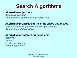
Search Algorithms Alternative objectives: Reach any goal state Find a short or shortest path to a goal state Alternative properties of the state space and moves: Tree structured vs graph structured, cyclic/acyclic Weighted/unweighted edges Alternative programming paradigms: Recursive Iterative Iterative deepening Genetic algorithms CSE 415 -- (c) S. Tanimoto, 2004 Search Algorithms

The Painted Squares Puzzle state: partially filled board. Initial state: empty board. Goal state: filled board, in which pieces satisfy all constraints. CSE 415 -- (c) S. Tanimoto, 2004 Search Algorithms

Recursive Depth-First Method Current board B  empty board. Remaining pieces Q  all pieces. Call Solve(B, Q). Procedure Solve(board B, set of pieces Q) For each piece P in Q, { For each orientation A { Place P in the first available position of B in orientation A, obtaining B’. If B’ is full and meets all constraints, output B’. If B’ is full and does not meet all constraints, return. Call Solve(B’, Q - {P}). } } Return. CSE 415 -- (c) S. Tanimoto, 2004 Search Algorithms

State-Space Graphs with Weighted Edges Let S be space of possible states. Let (si, sj) be an edge representing a move from si to sj. w(si, sj) is the weight or cost associated with moving from si to sj. The cost of a path [ (s1, s2), (s2, s3), . . ., (sn-1, sn) ] is the sum of the weights of its edges. A minimum-cost path P from s1 to sn has the property that for any other path P’ from s1 to sn, cost(P)  cost(P’). CSE 415 -- (c) S. Tanimoto, 2004 Search Algorithms

Uniform-Cost Search A more general version of breadth-first search. Processes states in order of increasing path cost from the start state. The list OPEN is maintained as a priority queue. Associated with each state is its current best estimate of its distance from the start state. As a state si from OPEN is processed, its successors are generated. The tentative distance for a successor sj of state si is computed by adding w(si, sj) to the distance for si. If sj occurs on OPEN, the smaller of its old and new distances is retained. If sj occurs on CLOSED, and its new distance is smaller than its old distance, then it is taken off of CLOSED, put back on OPEN, but with the new, smaller distance. CSE 415 -- (c) S. Tanimoto, 2004 Search Algorithms

Ideal Distances in A* Search Let f(s) represent the cost (distance) of a shortest path that starts at the start state, goes through s, and ends at a goal state. Let g(s) represent the cost of a shortest path from the start state to s. Let h(s) represent the cost of a shortest path from s to a goal state. Then f(s) = g(s) + h(s) During the search, the algorithm generally does not know the true values of these functions. CSE 415 -- (c) S. Tanimoto, 2004 Search Algorithms

Estimated Distances in A* Search Let g’(s) be an estimate of g(s) based on the currently known shortest distance from the start state to s. Let the h’(s) be a heuristic evaluation function that estimates the distance (path length) from s to the nearest goal state. Let f’(s) = g’(s) + h’(s) Best-first search using f’(s) as the evaluation function is called A* search. CSE 415 -- (c) S. Tanimoto, 2004 Search Algorithms

Admissibility of A* Search Under certain conditions, A* search will always reach a goal state and be able to identify a shortest path to that state as soon as it arrives there. The conditions are: h’(s) must not exceed h(s) for any s. w(si, sj) > 0 for all si and sj. This property of being able to find a shortest path to a goal state is known as the admissibility property of A* search. Sometimes we say that a particular A* algorithm is admissible. We can say this when its h’ function satisfies the underestimation condition and the underlying search problem involves positive weights. CSE 415 -- (c) S. Tanimoto, 2004 Search Algorithms

Search Algorithm Summary Unweighted graphsWeighted graphs blind search Depth-first Depth-first Breadth-first Uniform-cost uses heuristics Best-first A* CSE 415 -- (c) S. Tanimoto, 2004 Search Algorithms

Search Algorithms