WP6: CD Airfoil Test-case Experimental and numerical data base
430 likes | 652 Views
WP6: CD Airfoil Test-case Experimental and numerical data base. S. Moreau VEC Manager of the Fan System Core Competencies Manager of the Group Simulation Competency Center. October 200 8. ECL Experimental Set-up, LMFA. RMP. 11. RMP. 26. Thickness 4%. Camber 12°.

WP6: CD Airfoil Test-case Experimental and numerical data base
E N D
Presentation Transcript
WP6: CD Airfoil Test-case Experimental and numerical data base S. Moreau VEC Manager of the Fan System Core Competencies Manager of the Group Simulation Competency Center October 2008
ECL Experimental Set-up, LMFA RMP 11 RMP 26 Thickness 4% Camber 12° Open-Jet Aeroacoustic Experiment in ECL Large Wind Tunnel Airfoil chord length ~10 cm Valeo CD and NACA12 airfoils, Flat Plate, V2 and V3 airfoils Nozzle exit section 50 cm x 25 cm
CD Airfoil Experimental Data Base q • Valeo CD Airfoil: Re 1.5 105 ; M 0.05 ; several angles of attack (8° focus) • Far field noise measurements:Noise spectra and directivities • Remote Microphone Probe (RMP) measurements: Wall pressure statistics (Cp, frequency spectra, coherence, phase) • Hot wire measurements: Velocity statistics (mean and RMS velocity components, Reynolds stress and frequency spectra) Open-Jet Aeroacoustic Experiment in ECL Large Wind Tunnel Moreau et al, AIAA J. 2004, 2005, JFE 2005
Experimental Far Field Noise CD airfoil in high loading conditions Flat plate at zero angle of attack Spectrum Directivity q Evidence of 2 mechanisms: vortex-shedding noise and trailing-edge noise
Experimental Wall Pressure Statistics Wall pressure fluctuations must be statistically homogeneous f-5 is deduced from coherence measurements is deduced from the phase diagrams of streamwise cross spectra Equivalent Corcos’ model Gaussian model proposed (Roger & Moreau, AIAA 2002-2460).
Hot Wire Measurements Overview Wake Zoom Shear layer survey Inlet survey LES bc survey
Flow Visualization on CD Airfoil Separation bubble Direction of the flow laminar Suction side streaklines leading edge separation line turbulent Reattachment of the flow « Oil » Flow Tuft Film MVI_9612.avi Evidence of laminar flow separation at the leading edge Possible flow separation at the trailing edge
Numerical Wall Pressure Coefficient Two families of results k-w, SST and V2F k-e TL and WL Moreau et al, AIAA J. 2003
Numerical Wall Friction Coefficient Two families of results k-w, SST and V2F k-e TL and WL Moreau et al, AIAA J. 2003
Comparison of Wall Pressure Coefficients SST model Good prediction of laminar flow separation at the leading edge No prediction of onset of trailing edge flow separation
Broadband Models: Generalized Amiet - 1 • 3 main mechanisms considered: • Tip and leakage flow are not considered yet 2 - Trailing edge noise 1 - Turbulence-interaction noise 3 - Vortex-shedding noise
Broadband Models: Generalized Amiet - 2 Inflow velocity statistics Spanwise correlation length wall-pressure spectrum Radiation integrals (including back-scattering correction) • Turbulence Interaction Noise: • Trailing Edge Noise:
Stanford LES Set-up & Averaged Results • Choose the largest jet width (w = 50 cm) • LES domain in the jet core, with velocity B.C.'s coming from RANS (only mean values) • Better prediction of leading edge flow (Cp) with LES
Grid for Stanford LES Stanford Reference LES grid in 2D slice (2003) Very regular, fine and orthogonal grid at LE • Single block-structured topology • Grid Size: 960 x 84 x64 5.2 million nodes • Domain Size: (4 x 2.5 x0.1) x chord (first LES able to resolve the spanwise coherence length)
Grid Quality/Parameters of Stanford LES • Almost a DNS resolution in the normal direction • Very regular and orthogonal grid near airfoil • Grid independence of the solution verified on pressure spectra • Energy-conserving hybrid finite-difference/spectral code • Dynamic sub-grid-scale model
Stanford LES Instantaneous Results Leading-edge separation leading to transition on suction side Laminar boundary-layer on pressure side Qualitative agreement with experimental observation
2D vs 3D LES Instantaneous Results NACA0012 Re ~ 5-9 105 and M~0.2 3D 2D Drastic change of flow topology after transition
Stanford Broadband Noise (BBN) Sources Experiment LES Excellent qualitative and quantitative agreement
Stanford BBN Prediction Acoustic Analogies based on wall pressure statistics (Amiet) and on velocity statistics near the trailing edge (Ffowcs-Williams and Hall) Good agreement of both analogies with experimental data Effect of finite-chord up to 2 kHz Discrepancy between the two analogies at high frequencies
Evaluation of Other Unsteady Methods Starting from the same “LES domain” with the same RANS boundary conditions and, if possible, the same LES grid: Unsteady RANS: no unsteadiness was observed Detached Eddy Simulations (DES-SA within Fluent 6.1) Lattice Boltzmann (RANS/DNS) > Powerflow (EXA) LES with Immersed Boundary Technique Moreau et al, CTR Summer Program 2004
Grid and Simulation Parameters of SP-2004 • LBM:Powerflow 6.1.22 (3ddp) • Grid: 73551 voxels and 1491 surfels in a 2D slice (~1.2 M in 3D) • Smallest cell at LE is similar to body-fitted LES • Model: RANS k-e in 2D - No model in 3D • Simulation parameters: (Re=1.5 105) Time step: Dt =2.0e-7 CPU time for 100 time steps: 5 minutes on SGI Octane (1 CPU) • LES-IB: Structured Cartesian (PhD: S. Kang) • Grid: 4.8M in 3D (0.15M in a 2D slice) • Smallest cell at LE is ~2.5 larger than body-fitted LES • Model: LES + Dynamic Procedure • Simulation parameters: (Re=1.5 105) Time step: Dt =1.0e-4 CPU time for 100 time steps: 20 minutes on Linux cluster (8 CPU) Moreau et al, CTR Summer Program 2004
SP-2004 (Stanford) Grids Reference LES DES-SA 1-2 coarsening LBM-DNS LES-IB
SP-2004 (Stanford) Flow field Results Instantaneous Velocity Field Reference LES DES-SA LES-IB LBM-DNS
SP-2004 (Stanford) Wall Pressure Coefficient Only IB-LES provided a complete flow field close to reference LES Moreau et al, CTR Summer Program 2004
SP-2004 (Stanford) Wake Velocity Profiles X-wire Two coarse grids in any of the new simulations to yield good wake Moreau et al, CTR Summer Program 2004
SP-2004 (Stanford) Flow field Results DES gives unrealistic flow field (over production of k at LE) Grids for IB-LES need to re-visited for better TE prediction All over estimate the pressure fluctuations at low frequencies
STAR-CD LES Simulations (2005-2006) PISO algorithm for time discretization Central differencing and upwind MARS scheme (no stable solution could be obtained even in 2D with CDS for all grid topologies tested). To keep a CFL number below 1 throughout the computational domain, a maximum allowable time step Dt = 1.5 10-5 s is used. 5 to 10 time units run to eliminate the transient and collect reliable statistics (based on the free stream velocity of 16 m/s). Smagorinsky sub-grid scale (SGS) model together with a van Driest near-wall damping and WALE SGS are used. k-e based DES is selected. Moreau et al, AIAA 2005-2916 Evaluation of different numerical Schemes Evaluation of different SGS models Re-assessment of the DES model with a different code
Final MARS LES Grid Topology (2005) Zoom LE Zoom TE 1,115,000 cells • Similar grid 1-2 coarsening as DES with Fluent 6.1 • Only 5% chord span • Good near-surface resolution: Dx+≤ 20 ; Dy+≤ 1 ; Dz+≤ 10
MARS LES Instantaneous Velocity Field STAR-CD MARS LES Stanford Reference LES Similar small structures created after separation convected downstream towards the trailing edge Larger flow separation at the leading edge in MARS LES. More coherent structures at the trailing edge in MARS LES.
MARS LES Wall Pressure Coefficient Qualitative agreement on the laminar separation bubble (good level of pressure plateau but too large extent of the bubble, 11.2% instead of 3.7%) First simulation to predict the positive pressure gradient up to mid-chord.
MARS LES Wake Velocity Profiles Excellent agreement in the near wake for the MARS LES Too large diffusion and deflection of the wake in the DES.
MARS LES Wall Pressure Spectra No homogeneous statistics close to TE P2 P60: mid-chord (-60 mm) P14: -14 mm P8: -8 mm P2: -2 mm Origin: TE P8 P60 P14 • Too large structures and coherence at the trailing edge • Fluctuations are getting damped towards TE (MARS upwinding) Too high levels everywhere
MARS Fine Scale Structures Iso-values of normalized Q colored by the streamwise vorticity Turbulent re-attach. Turbulent T.E.Separation Laminar L.E. separation Larger structures than reference LES
DES Simulation Issue Well attached flow field all the way to the trailing edge as in RANS simulations Short laminar separation bubble is not captured Transition occurs at the stagnation point (local turbulent kinetic energy overproduction in k-e model). Sub-grid Turbulent Viscosity Velocity Field
Conclusions Summer 2005 The STAR-CD MARS LES reproduces all qualitative features of the flow encountered in the ECL experiment and simulated in the reference LES (Wang et al, Stanford 2004). A short laminar separation bubble is formed, reattaches and sheds small vortices that are convected towards the trailing edge. Evolution of the boundary layer seems to be well captured, especially the experimental positive pressure gradient up to mid-chord. Yet the laminar separation bubble is too wide and the wall pressure fluctuations are damped at the trailing edge (most likely due to MARS upwind scheme).No use for self-noise prediction. All DES found inadequate for this attached flow (transitional airfoil with a short laminar bubble). Further grid optimization required to remove instabilities with Central Differencing Scheme (CDS).
Final CDS LES Grid Topology (2006) D. Laurence, VKI Lecture Series 2005 Y. Addad, PhD UMIST 690,000 cells • 3-4 grid coarsening in all directions • 10% chord span • Good near-surface resolution: Dx+~ 2.5 ; Dy+~ 2 ; Dz+~ 3.6 3-4 coarsening Stability of CD scheme without significant oscillations Only a small jump in the turbulent viscosity
CDS LES Wall Pressure Coefficient Same qualitative agreement on the laminar separation bubble No significant differences between the two SGS models
CDS LES Wake Velocity Profiles Same excellent agreement in the near wake for the CDS-LES No significant differences between the two SGS models
CDS LES Wall Pressure Spectra Good overall predicition with the CD SGS model has only a moderate effect on spectra
CDS Fine Scale Structures Iso-values of normalized Q colored by the streamwise vorticity t = 0.07 s t = 0.25 s Smaller structures than with MARS scheme
SP-2006 (Stanford) Unstructured LES <4% difference Excellent agreement with both structured LES and experimental data
Conclusions Summer 2006 The STAR-CD CDS LES improves the MARS LES significantly (over dissipative in the TE region) and compares favorably with the ECL experiment and the reference LES (Wang et al, Stanford 2004). A regular grid with smooth jumps is required if coarsening is to be used to yield numerical stability and limited oscillations. (3-4) coarsening as suggested by Laurence seems to provide the best compromise and still yield reasonable grid sizes (< 1 Million nodes). Different SGS models do not yield significant differences Unstructured LES solver (CDP, Stanford) with the same numerical schemes and SGS as the reference structured LES yields similar results . But all LES still show weaknesses in the laminar flow recirculation and especially in the transition process (we have as many bubble sizes as LES) Yet in the trailing edge region, similar statistics are achieved and consequently same broadband noise prediction