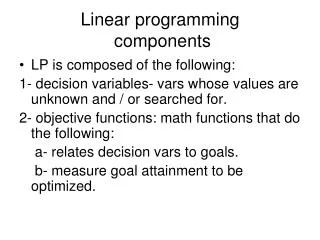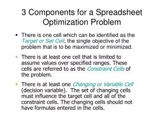
3 Components for a Spreadsheet Linear Programming Problem
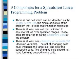
3 Components for a Spreadsheet Linear Programming Problem. There is one cell which can be identified as the Target or Set Cell , the single objective of the problem that is to be maximized or minimized.

3 Components for a Spreadsheet Linear Programming Problem
E N D
Presentation Transcript
3 Components for a Spreadsheet Linear Programming Problem • There is one cell which can be identified as the Target or Set Cell, the single objective of the problem that is to be maximized or minimized. • There is at least one cell that is limited to assume values over specified ranges. These cells are referred to as the Constraint Cells of the problem. • There is at least one Changing or Variable Cell (decision variable). The set of changing cells must influence the target cell and all of the constraint cells. The changing cells should not have formulas entered in the cells.
3 Steps of Linear Programming • Model Formulation • Spreadsheet Based • Algebraic • Model Solution • Graphical Analysis (for 2 decision variable problems) • Simplex Method • Excel Solver • Sensitivity Analysis
Product Mix Algebraic Formulation Maximize 5000 E9 + 4000 F9 Subject to 10 E9 + 15 F9 <= 150 (dept A hours) 20 E9 + 10 F9 <= 160 (dept B hours) 30 E9 + 10 F9 >= 135 (testing hours) E9 >= 1 (current order) F9 >= 3 (current order) where E9,F9 represent the quantity to produce next period of each model
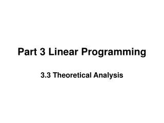
Important LP Terminology • Linear functions are functions in which each variable appears in a separate term raised to the first power and multiplied by a constant, which may be 0. • A feasible solution is an assignment of values to the decision variables that satisfies all the problem's constraints. • The objective does not affect the feasibility of the problem. • An optimal solution is a feasible solution that results in the largest possible objective function value, z, when maximizing or smallest z when minimizing
Graphical Solutions • Plot all constraints including nonnegativity ones • Determine the feasible region. (The feasible region is the set of feasible solution points) • Identify the optimal solution using either • the level curve method • the extreme point method
Feasible Regions • The feasible region for a two-variable linear programming problem can be nonexistent, a single point, a line, a polygon, or an unbounded area. • Assuming that a feasible region exists, an optimal solution will always occur at one or more of the extreme points, where an extreme point is a corner point of the feasible region. • If a constraint can be removed without affecting the shape of the feasible region, the constraint is said to be redundant. • A linear program which is overconstrained so that no point satisfies all the constraints is said to be infeasible.
Level Curves • Plot a level curve for a targeted objective function value • Level curves are parallel lines that shift away from the origin as the targeted objective function value increases • Slide the level curve in the direction of improvement (away from the origin if maximizing, toward the origin if minimizing) until it reaches the last point where it still touches at least one point in the feasible region • Solve the two equations which specify the identified feasible point to determine the optimal solution
Extreme Point (3.5, 3) (6.5, 3) (4.5, 7) (1.5, 9) ¶=5000E9 + 4000F9 $29,500 $44,500 $50,500 $43,500 Extreme Point Method
Example: Infeasible Problem • Solve graphically for the optimal solution: Max z = 2x1 + 6x2 s.t. 4x1 + 3x2< 12 2x1 + x2> 8 x1, x2> 0
x2 2x1 + x2> 8 8 4x1 + 3x2< 12 4 x1 3 4 Example: Infeasible Problem • There are no points that satisfy both constraints, hence this problem has no feasible region, and no optimal solution.
Solver Result Message • Solver could not find a feasible solution • Possible problems: • too many constraints • one of the constraints may be entered wrong (e.g. the inequality sign might be going the wrong way) • you may not have the correct changing cells (decision variables) specified • one or more formulas in the spreadsheet may have been erased.
Types of LP Solutions • Any linear program falls in one of three categories: • is infeasible • has a unique optimal solution or alternate optimal solutions • has an objective function that can be increased without bound • In the graphical method, if the objective function line is parallel to a boundary constraint in the direction of optimization, there are alternate optimal solutions, with all points on this line segment being optimal.
Solver Result Messages • Solver found a solution. All constraints and optimality conditions are satisfied: Solver has correctly identified an optimal solution for the problem you have formulated. Note that there may be alternative optimal solutions possible however. • Solver has converged to the current solution. All constraints are satisfied: You have not selected the linear programming option in the Solver options. Thus nonlinear programming is being performed and this is the best solution Solver has found so far. It is not guaranteed to be the optimal one however.
Example: Unbounded Problem • Solve graphically for the optimal solution: Max z = 3x1 + 4x2 s.t. x1 + x2> 5 3x1 + x2> 8 x1, x2> 0
x2 3x1 + x2> 8 8 x1 + x2> 5 5 Max 3x1 + 4x2 x1 2.67 5 Example: Unbounded Problem • The feasible region is unbounded and the objective function line can be moved parallel to itself without bound so that z can be increased infinitely.
Solver Result Messages • Set Cell values do not converge:Your model as formulated is unbounded. One or more constraint is missing from the problem or entered wrong (e.g. an inequality sign is in the wrong direction). Often times the modeler has forgotten to check the Assume Nonnegativity option in Solver. • Note: A feasible region may be unbounded and yet there may be optimal solutions. This is common in minimization problems and is possible in maximization problems. In these cases, you will see the optimal Solver solution message.
Solver Result Messages • The conditions for Assume Linear Model are not satisfied: Solver’s preliminary tests indicate that your model is not linear. • This may be the case. However sometimes this message occurs due to poor scaling (e.g. some #s are in % and others in millions). If you think your model is linear, try resolving the model again. Often times Solver can find the solution the second time. If not, use the Use Automatic Scaling option in Solver. Solver will attempt to rescale your data. If that doesn’t solve the problem, you can try rescaling the data yourself.
Solver Modeling Requirements • All components of the optimization problem must be on the same worksheet. Solver’s settings are saved with the sheet. • Solver’s constraint dialog box will not let you enter formulas. All formulas and calculations must be done on the worksheet. The constraint dialog box just compares cells to determine feasibility.
Goals For Spreadsheet Design • Communication - A spreadsheet's primary business purpose is that of communicating information to managers. • Reliability - The output a spreadsheet generates should be correct and consistent. • Auditability - A manager should be able to retrace the steps followed to generate the different outputs from the model in order to understand the model and verify results. • Modifiability - A well-designed spreadsheet should be easy to change or enhance in order to meet dynamic user requirements.
Spreadsheet Design Guidelines • Organize the data, then build the model around the data. • Do not embed numeric constants in formulas! • Things which are logically related should be physically related. • Use formulas that can be copied. • Column/rows totals should be close to the columns/rows being totaled. • The English-reading eye scans left to right, top to bottom. • Use color, shading, borders and protection to distinguish changeable parameters from other model elements. • Use text boxes and cell notes to document various elements of the model.
Network Of Routes 120 Amsterdam (500) Leipzig (400) 130 62 41 Nancy(900) 61 40 Antwerp (700) 100 110 Liege (200) 90 102.5 122 Le Havre (800) Tilburg (500) 42
The Transportation Tableau To Supply Leipzig Nancy Liege From Tilburg 120 130 41 62 500 Amsterdam 61 40 100 110 700 Antwerp 102.5 90 122 42 800 Le Havre Demand 400 900 200 500