Download
1 / 89
1.08k likes | 3.36k Views
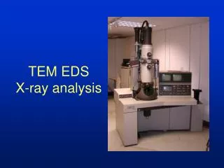
TEM EDS X-ray analysis. Topics. EDS Hardware TEM EDS vs. SEM EDS Signal Processing and Quantification k-factor determination and uncertainty CM200 and EDAX Genesis software. EDS unit. Oxford Instruments: EDSHardwareExplained.pdf www.x-raymicroanalysis.com.

E N D
Topics • EDS Hardware • TEM EDS vs. SEM EDS • Signal Processing and Quantification • k-factor determination and uncertainty • CM200 and EDAX Genesis software
EDS unit Oxford Instruments: EDSHardwareExplained.pdf www.x-raymicroanalysis.com Image courtesy of Oxford Instruments
Si(Li) crystal FET Window Electron trap (SEM only) Collimator EDS detector (SEM) Image courtesy of Oxford Instruments
TEM detector Image courtesy of Oxford Instruments
Silicon Drift Detector Peltier Cooler Heatsink Heat pipe Image courtesy of Oxford Instruments
SDD Window Electron trap FET SDD Collimator Image courtesy of Oxford Instruments
SDD detail Image courtesy of Oxford Instruments
X-ray Generation and Detection • The number of X-rays generated is the product of • the number of electrons * • number of atoms * • ionization cross-section (s) * • fluorescent yield (w). • The number of X-rays we detect is reduced by absorption of the X-rays in the sample and detector and by the limited solid angle subtended by the detector. (ignoring fluorescence effects)
Ionization cross-section Bethe cross-section model U = (E0/Ec) = overvoltage
Avoid this range of U (mostly SEM issue) Ionization Cross-section vs. Overvoltage Overvoltage values (U) for 120kV beam
C O Na Detector Efficiency - UTW vs. Be Window
TEM vs. SEM • Higher kV in TEM • Hard X-rays • High energy BSE (can’t use electron trap) • Ill-defined TEM sample geometry • Thin TEM sample vs. thick (semi-infinite)
Revised Goldstein Equation b = broadening (m) E0 = Beam energy in keV Z = Atomic Number Nv = atoms per volume (#/m3) t = thickness (m) W&C eq 36.1
Sample geometry • An SEM sample is usually assumed to be a flat, homogeneous, semi-infinite object. • TEM samples vary in thickness and can be bent.
Pt Obj aperture TEM EDS geometry
Qualitative Analysis • Match families of peaks • Start at higher energies and work down • Be careful of spectral contamination (e.g. Cu from grid) • Be careful when using Auto Peak ID functions.
Quantification • Extract peak intensities • Remove Background • Deconvolve overlapped peaks if needed • Quantify with Cliff-Lorimer equation • Modify results with absorption & fluorescence corrections
Extract intensity • Straight line subtraction • Kramers Law continuum modeling • “Top Hat” filtering
Background modeling • Need to choose background areas • Requires knowledge of detector response (esp. at low keV)
Linear combination Where Si are pure element standard spectra To calculate the ci, perform a multiple least squares fit and minimize the c2 value. You multiply the intensity of the Si by ci to get the peak intensities.
Cliff-Lorimer equation Ca & Cb are in weight percent (a tradition started by Castaing)
Cliff-Lorimer equation • C-L equation describes relative concentrations and gives only n-1 equations for n elements • The nth equation is to require the sum of the concentrations = 1. If you neglect an element, the calculated concentrations will vary from the true concentrations though the relative amounts are OK. • The C-L equation neglects absorption and fluorescence. It is exactly valid only in the thin film limit (i.e. at t = 0).
k-factors • kab-factors are relative sensitivity factors. Always reported with respect to another (usually common) element. • The original reference element was Si because Cliff and Lorimer were geologists. Metallurgists will often use Fe. • We can use theoretical k-factors, but …
Theoretical kTiFe can vary by over 10% Theoretical k-factors
k-factors • We can use theoretical k-factors, but … experimental k-factors are more reliable. • Experimental k-factors will be valid for the instrument and the conditions used for the acquisition ONLY. • A change in microscope or detector parameters will change the k-factors (e.g. detector icing, radiation damage, etc.)
Experimental k-factors • Ia/Ib will vary with thickness due to absorption and fluorescence. • Since the k-factors are exact only in the thin-film limit, we can measure the ratios at various thicknesses and extrapolate to zero thickness.
Thickness determination • Can measure crystalline thickness using CBED techniques. • Can use EELS to measure material thickness though the mean-free-path (l) needs to be determined first. • Contamination marks, projections of defects, and stereo imaging have also been used.
van Capellen technique • If you assume a constant beam current and moderate absorption, then the count rate scales with thickness. • Plot the ratio against the sum of the counts rather than thickness. • Extrapolate to zero count rate (i.e. zero thickness). • Do a linear regression to get the Y-intercept. • Most packages will give you a standard estimate of error (i.e. s).