Sorting Algorithms

1. Sorting Algorithms AnanthGrama, Anshul Gupta, George Karypis, and Vipin Kumar Adapted for 3030 To accompany the text ``Introduction to Parallel Computing'', Addison Wesley, 2003.

2. Topic Overview • Issues in Sorting on Parallel Computers • Sorting Networks • Bubble Sort and its Variants • Quicksort • Bucket and Sample Sort • Other Sorting Algorithms

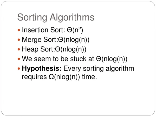
3. Sorting: Overview • One of the most commonly used and well-studied kernels. • Sorting can be comparison-based or noncomparison-based. • The fundamental operation of comparison-based sorting is compare-exchange. • The lower bound on any comparison-based sort of n numbers is Θ(nlog n) . • We focus here on comparison-based sorting algorithms.

4. Sorting: Basics What is a parallel sorted sequence? Where are the input and output lists stored? • We assume that the input and output lists are distributed. • The sorted list is partitioned with the property that each partitioned list is sorted and each element in processor Pi's list is less than that in Pj's list if i < j.

5. Sorting: Basics What is the parallel counterpart to a sequential comparator? • If each processor has one element, the compare exchange operation stores the smaller element at the processor with smaller id. This can be done in ts + tw time. • If we have more than one element per processor, we call this operation a compare split. Assume each of two processors have n/p elements. • After the compare-split operation, the smaller n/p elements are at processor Pi and the larger n/p elements at Pj, where i < j. • The time for a compare-split operation is (ts+ twn/p), assuming that the two partial lists were initially sorted.

6. Sorting Networks • Networks of comparators designed specifically for sorting. • A comparator is a device with two inputs x and y and two outputs x' and y'. For an increasing comparator, x' = min{x,y} and y' = min{x,y}; and vice-versa. • We denote an increasing comparator byand a decreasing comparator by Ө. • The speed of the network is proportional to its depth.

7. Sorting Networks: Comparators A schematic representation of comparators: (a) an increasing comparator, and (b) a decreasing comparator.

8. Sorting Networks A typical sorting network. Every sorting network is made up of a series of columns, and each column contains a number of comparators connected in parallel.

9. Sorting Networks: Bitonic Sort • A bitonic sorting network sorts n elements in Θ(log2n) time. • A bitonic sequence has two tones - increasing and decreasing, or vice versa. Any cyclic rotation of such networks is also considered bitonic. • 1,2,4,7,6,0 is a bitonic sequence, because it first increases and then decreases. 8,9,2,1,0,4 is another bitonic sequence, because it is a cyclic shift of 0,4,8,9,2,1. • The kernel of the network is the rearrangement of a bitonic sequence into a sorted sequence.

10. Sorting Networks: Bitonic Sort • Let s = a0,a1,…,an-1 be a bitonic sequence such that a0 ≤ a1 ≤ ··· ≤ an/2-1 and an/2 ≥an/2+1 ≥ ··· ≥ an-1. • Consider the following subsequences of s: s1 = min{a0,an/2},min{a1,an/2+1},…,min{an/2-1,an-1} s2 = max{a0,an/2},max{a1,an/2+1},…,max{an/2-1,an-1} (1) • Note that s1 and s2 are both bitonic and each element of s1 is less than every element in s2. • We can apply the procedure recursively on s1 and s2 to get the sorted sequence.

11. Sorting Networks: Bitonic Sort Merging a 16-element bitonic sequence through a series of log 16 bitonic splits.

12. Sorting Networks: Bitonic Sort • We can easily build a sorting network to implement this bitonic merge algorithm. • Such a network is called a bitonic merging network. • The network contains log n columns. Each column contains n/2 comparators and performs one step of the bitonic merge. • We denote a bitonic merging network with n inputs by BM[n]. • Replacing the  comparators by Ө comparators results in a decreasing output sequence; such a network is denoted by ӨBM[n].

13. Sorting Networks: Bitonic Sort A bitonic merging network for n = 16. The input wires are numbered 0,1,…, n - 1, and the binary representation of these numbers is shown. Each column of comparators is drawn separately; the entire figure represents a BM[16] bitonic merging network. The network takes a bitonic sequence and outputs it in sorted order.

14. Sorting Networks: Bitonic Sort How do we sort an unsorted sequence using a bitonic merge? • We must first build a single bitonic sequence from the given sequence. • A sequence of length 2 is a bitonic sequence. • A bitonic sequence of length 4 can be built by sorting the first two elements using BM[2] and next two, using ӨBM[2]. • This process can be repeated to generate larger bitonic sequences.

15. Sorting Networks: Bitonic Sort A schematic representation of a network that converts an input sequence into a bitonic sequence. In this example, BM[k] and ӨBM[k] denote bitonic merging networks of input size k that use  and Ө comparators, respectively. The last merging network (BM[16]) sorts the input. In this example, n = 16.

16. Sorting Networks: Bitonic Sort The comparator network that transforms an input sequence of 16 unordered numbers into a bitonic sequence.

17. Sorting Networks: Bitonic Sort • The depth of the network is Θ(log2n). • Each stage of the network contains n/2 comparators. A serial implementation of the network would have complexity Θ(nlog2n).

18. Performance of Parallel Bitonic Sort The performance of parallel formulations of bitonic sort for n elements on p processes.

19. Bubble Sort and its Variants The sequential bubble sort algorithm compares and exchanges adjacent elements in the sequence to be sorted: Sequential bubble sort algorithm.

20. Bubble Sort and its Variants • The complexity of bubble sort is Θ(n2). • Bubble sort is difficult to parallelize since the algorithm has no concurrency. • A simple variant, though, uncovers the concurrency.

21. Odd-Even Transposition Sequential odd-even transposition sort algorithm.

22. Odd-Even Transposition Sorting n = 8 elements, using the odd-even transposition sort algorithm. During each phase, n = 8 elements are compared.

23. Odd-Even Transposition • After n phases of odd-even exchanges, the sequence is sorted. • Each phase of the algorithm (either odd or even) requires Θ(n) comparisons. • Serial complexity is Θ(n2).

24. Parallel Odd-Even Transposition • Consider the one item per processor case. • There are n iterations, in each iteration, each processor does one compare-exchange. • The parallel run time of this formulation is Θ(n). • This is cost optimal with respect to the base serial algorithm but not the optimal one.

25. Parallel Odd-Even Transposition Parallel formulation of odd-even transposition.

26. Parallel Odd-Even Transposition • Consider a block of n/p elements per processor. • The first step is a local sort. • In each subsequent step, the compare exchange operation is replaced by the compare split operation. • The parallel run time of the formulation is

27. Parallel Odd-Even Transposition • The parallel formulation is cost-optimal for p = O(log n). • The isoefficiency function of this parallel formulation is Θ(p2p).

28. Quicksort • Quicksort is one of the most common sorting algorithms for sequential computers because of its simplicity, low overhead, and optimal average complexity. • Quicksort selects one of the entries in the sequence to be the pivot and divides the sequence into two - one with all elements less than the pivot and other greater. • The process is recursively applied to each of the sublists.

29. Quicksort The sequential quicksort algorithm.

30. Quicksort Example of the quicksort algorithm sorting a sequence of size n = 8.

31. Quicksort • The performance of quicksort depends critically on the quality of the pivot. • In the best case, the pivot divides the list in such a way that the larger of the two lists does not have more than αnelements (for some constant α). • In this case, the complexity of quicksort is O(nlog n).

32. Parallelizing Quicksort • Lets start with recursive decomposition - the list is partitioned serially and each of the subproblems is handled by a different processor. • The time for this algorithm is lower-bounded by Ω(n)! • Can we parallelize the partitioning step - in particular, if we can use n processors to partition a list of length n around a pivot in O(1) time, we have a winner. • This is difficult to do on real machines, though.

33. Parallelizing Quicksort: PRAM Formulation • We assume a CRCW (concurrent read, concurrent write) PRAM with concurrent writes resulting in an arbitrary write succeeding. • The formulation works by creating pools of processors. Every processor is assigned to the same pool initially and has one element. • Each processor attempts to write its element to a common location (for the pool). • Each processor tries to read back the location. If the value read back is greater than the processor's value, it assigns itself to the `left' pool, else, it assigns itself to the `right' pool. • Each pool performs this operation recursively. • Note that the algorithm generates a tree of pivots. The depth of the tree is the expected parallel runtime. The average value is O(log n).

34. Parallelizing Quicksort: PRAM Formulation A binary tree generated by the execution of the quicksort algorithm. Each level of the tree represents a different array-partitioning iteration. If pivot selection is optimal, then the height of the tree is Θ(log n), which is also the number of iterations.

35. Parallelizing Quicksort: PRAM Formulation The execution of the PRAM algorithm on the array shown in (a).

36. Parallelizing Quicksort: Shared Address Space Formulation • Consider a list of size n equally divided across p processors. • A pivot is selected by one of the processors and made known to all processors. • Each processor partitions its list into two, say Li and Ui, based on the selected pivot. • All of the Li lists are merged and all of the Ui lists are merged separately. • The set of processors is partitioned into two (in proportion of the size of lists L and U). The process is recursively applied to each of the lists.

37. Shared Address Space Formulation

38. Parallelizing Quicksort: Shared Address Space Formulation • The only thing we have not described is the global reorganization (merging) of local lists to form L and U. • The problem is one of determining the right location for each element in the merged list. • Each processor computes the number of elements locally less than and greater than pivot. • It computes two sum-scans to determine the starting location for its elements in the merged L and U lists. • Once it knows the starting locations, it can write its elements safely.

39. Parallelizing Quicksort: Shared Address Space Formulation Efficient global rearrangement of the array.

40. Parallelizing Quicksort: Shared Address Space Formulation • The parallel time depends on the split and merge time, and the quality of the pivot. • The latter is an issue independent of parallelism, so we focus on the first aspect, assuming ideal pivot selection. • The algorithm executes in four steps: (i) determine and broadcast the pivot; (ii) locally rearrange the array assigned to each process; (iii) determine the locations in the globally rearranged array that the local elements will go to; and (iv) perform the global rearrangement. • The first step takes time Θ(log p), the second, Θ(n/p) , the third, Θ(log p) , and the fourth, Θ(n/p). • The overall complexity of splitting an n-element array is Θ(n/p) + Θ(log p).

41. Parallelizing Quicksort: Shared Address Space Formulation • The process recurses until there are p lists, at which point, the lists are sorted locally. • Therefore, the total parallel time is: • The corresponding isoefficiency is Θ(plog2p) due to broadcast and scan operations.

42. Parallelizing Quicksort: Message Passing Formulation • A simple message passing formulation is based on the recursive halving of the machine. • Assume that each processor in the lower half of a p processor ensemble is paired with a corresponding processor in the upper half. • A designated processor selects and broadcasts the pivot. • Each processor splits its local list into two lists, one less (Li), and other greater (Ui) than the pivot. • A processor in the low half of the machine sends its list Ui to the paired processor in the other half. The paired processor sends its list Li. • It is easy to see that after this step, all elements less than the pivot are in the low half of the machine and all elements greater than the pivot are in the high half.

43. Parallelizing Quicksort: Message Passing Formulation • The above process is recursed until each processor has its own local list, which is sorted locally. • The time for a single reorganization is Θ(log p) for broadcasting the pivot element, Θ(n/p) for splitting the locally assigned portion of the array, Θ(n/p) for exchange and local reorganization. • We note that this time is identical to that of the corresponding shared address space formulation. • It is important to remember that the reorganization of elements is a bandwidth sensitive operation.