Download
1 / 46
460 likes | 471 Views
Correlation & Regression. Chapter 15. Correlation. statistical technique that is used to measure and describe a relationship between two variables (X and Y). 3 Characteristics. 1. The direction of the relationship Positive correlation ( +) Negative Correlation (-).

E N D
Correlation & Regression Chapter 15
Correlation • statistical technique that is used to measure and describe a relationship between two variables (X and Y).
3 Characteristics • 1. The direction of the relationship • Positive correlation ( +) • Negative Correlation (-)
2. The Form of the Relationship • Relationships tend to have a linear relationship. A line can be drawn through the middle of the data points in each figure. • The most common use of regression is to measure straight-line relationships. • Not always the case
Scatterplot • Visual representation of scores. • Each individual score is represented by a single point on the graph. • Allows you to see any patterns of trends that exist in the data.
3. The Degree of the Relationship • Measures how well the data fit the specific form being considered. • The degree of relationship is measured by the numerical value of the correlation (0 to 1.00) • A perfect correlation is always identified by a correlation of 1.00 and indicates a perfect fit. • A correlation value of 0 indicates no fit or relationship at all.
Pearson Product-Moment Correlation • Measures the degree and the direction of the linear relationship between two variables • Identified by r degree to which X and Y vary together r= degree to which X and Y vary separately = ___covariability of X and Y____ variability of X and Y separately
How do we calculate the Pearson Correlation? • Sum of products of deviations: provides a parallel procedure for measuring the amount of covariability between two variables. Definitional formulaSP = (X-X) (Y-Y) XY Computational SP = XY - n formula
Computational Formula = SP r SSx SSy
Using and Interpreting r • Prediction • Validity • Reliability • Theory Verification *“CORRELATION DOES NOT MEAN CAUSATION”
Restriction of Range • Occurs whenever a correlation is computed from scores that do not represent the full range of possible values. • ie:IQ tests among college students. • Correlations should not be generalized beyond the range of data represented in the sample.
Other Correlation Coefficients • Spearman r • Two ranked (ordinal) variables • Point-biserial r • Pearson r between dichotomous and continuous variable • Phi Coefficient • Pearson r between two dichotomous variables
Outliers • An individual with X and/or Y values that are substantially different (larger or smaller) from the values obtained for the other individuals in the data set. • An outlier can dramatically influence the value obtained for the correlation. • Always look at scatter plots to determine if there are outliers.
Coefficient of Determination • r2 measures the proportion of variability in one variable that can be determined from the relationship with the other variable. • A correlation of r = .80 means that r2 = .64 or 64% of the variability in Y scores can be predicted from the relationship with X.
Hypothesis Testing with r • Standard hypotheses: • H0: r = 0 (There is no population correlation) • H1: r¹ 0 (There is a real correlation) • Other hypotheses are possible, e.g., one-sided hypotheses or hypotheses with r¹ 0. • If the alternative hypothesis prevails, one can state that a correlation is significant in the sample
There will always be some error between a sample correlation (r) and the population correlation () it represents. • Goal of the hypothesis test is to decide between the following two alternatives: • The nonzero sample correlation is simply due to chance. • The nonzero sample correlation accurately represents a real, nonzero correlation in the population. • USE TABLE B 6.
CAPA Example • Questions 5-10 • Step 1) Calculate the SS for X • Step 2) Calculate the SS for Y • Formula for SS: ( X)2 • SS = = (X-X2) OR SS= X2 - n
Calculation cont’d • Calculate XY to obtain Definitional formulaSP = (X-X) (Y-Y) or X Y Computational SP = XY - n formula
Calculate r: SP r= • Compare to Table B6 and find the critical value • What can we determine??????
Best Fitting Line • The line that gives the best prediction of Y • We must find the specific values for a and b SP b = SSx a = Y –bX Y = bX + a
Caution Be Aware • The predicted value is not perfect unless r = 1.00 or –1.00 • The regression equation should not be used to make predictions for X values that fall outside the range of values covered by the original data (restriction of range).
The Spearman Correlation • Used for non-linear relationships • Ordinal (ranked) Data • Can be used as an alternative to the Pearson • Measure of consistency
Ranks • Consistent relationships among scores produces a linear relationship when the scores are converted to ranks.
When is the Spearman correlation used? • When the original data are ordinal, when the X and Y values are ranks. • When a researcher wants to measure the consistency of a relationship between X and Y, independent of the specific form of the relationship. • monotonic
Calculating a Spearman Correlation Step 1) Rank X and Y scores (separately) Step 2) Use the Pearson correlation formula for the ranks of the X and Y scores. rs
Tied Scores • When converting scores into ranks for the Spearman correlation, there may be two or more identical scores. If this occurs: • List the scores in order from smallest to largest (include tied values) • Assign a rank (1st, 2nd ) to each position in the list. • When two or more scores are tied, compute the mean of their ranked positions, and assign this mean value as the final rank for each score.
Special Formula for the Spearman Correlation • X = (n+1)/2 • SS= n(n2 –1) 12 6D2 rs = 1– n(n2-1) *D is the difference between the X rank and the Y rank for each individual. *N = number of pairs
Regression • Is the statistical technique for finding the best-fitting straight line for a set of data. • To find the line that best describes the relationship for a set of X and Y data.
Regression Analysis • Question asked: Given one variable, can we predict values of another variable? • Examples: Given the weight of a person, can we predict how tall he/she is; given the IQ of a person, can we predict their performance in statistics; given the basketball team’s wins, can we predict the extent of a riot. ...
Using regression analysis one can make this type of prediction: • Predictor and Criterion • Regression analysis allows one to • Ø predict values of the criterion: point prediction • Øestimate strength of predictability (significance testing)
Regression line • makes the relationship between variables easier to see. • identifies the center, or central tendency, of the relationship, just as the mean describes central tendency for a set of scores. • can be used for a prediction.
The Equation for a Line Y = bX + a • b = the slope • a = y-intercept • Y= predicted value
Example • Local tennis club charges $5 per hour plus an annual membership fee of $25. • Compute the total cost of playing tennis for 10 hours per month. (predicted cost) Y = (constant)bX + (constant) a When X = 10 Y= $5(10 hrs) + $25 Y = 75
When X = 30 Y= $5(30 hrs) + $25 Y = $175
Least Squares Solution • Minimize the square root of the squared differences between data points and the line • The best fit line has the smallest total squared error • We seek to minimize (Y - Y)2
When estimating the parameters for slope and intercept, one minimizes the sum of the squared residuals, that is, prediction errors: • least squares estimation.
Equations • The line that gives the best prediction of Y • We must find the specific values for a and b SP b = SSx a = Y –bX Y = bX + a
Caution Be Aware • The predicted value is not perfect unless r = 1.00 or –1.00 • The regression equation should not be used to make predictions for X values that fall outside the range of values covered by the original data (restriction of range).
Conclusion • Using methods of statistical inference in regression analysis we ask whether the regression line explains a significant portion of the variance of Y.