Regression vs. Correlation
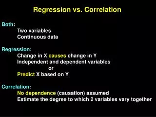
Regression vs. Correlation. Both : Two variables Continuous data Regression : Change in X causes change in Y Independent and dependent variables or Predict X based on Y Correlation : No dependence (causation) assumed Estimate the degree to which 2 variables vary together.

Regression vs. Correlation
E N D
Presentation Transcript
Regression vs. Correlation Both: Two variables Continuous data Regression: Change in X causes change in Y Independent and dependent variables or Predict X based on Y Correlation: No dependence (causation) assumed Estimate the degree to which 2 variables vary together
Regression & correlation often confused Give research examples of: Correlation- no causation implied Regression- state independent and dependent Regression- the trickier case where no dependence, but wish to make predictions
Simple linear regression --Two continuous variables --Linear relationship The most simple relationship between any 2 variables is a straight line Y= a + bX dependent variable dependent variable = intercept + slope * a is sample estimate of (population parameter) b is sample estimate of (population parameter)
Purpose of simple linear regression - Describe linear relationship between independent and dependent variables - Predict one variable bases on measurement of another when there is a linear relationship between the two
Y= a + bX dependent variable dependent variable = intercept + slope * You have: data for dependent (Y) and independent (X) variables You want to: --fit a line --calculate slope and intercept --determine if relationship is significant
How to fit the best line?? We want to fit a regression line that will allow us to estimate a value of Y for any given X Pictures first…….. Then math
hypothetical data- each point = 1 lake Chl a (ug/L; index of algae biomass) P concentration (ug/L)
Start with horizontal line at Ybar – essentially what you did in t test or ANOVA --The deviations from this line sum to 0 --the sum of squared deviations is smaller than for any other horizontal line Y bar Chl a (ug/L; index of algae biomass) P concentration (ug/L)
Tilted line gives smaller deviations find the one with smallest deviations: Least squares linear regression line Line provides Ŷ, an estimate of Y at any given X Chl a (ug/L; index of algae biomass) P concentration (ug/L)
Least squares linear regression line will pass through the means of X and Y– think of pivoting around this point Ybar Chl a (ug/L; index of algae biomass) Xbar P concentration (ug/L)
Minimize sum of squared deviations from line: (Y-Ŷ)2 = d2y*x = Sum of deviations from line = unexplained or residual sum of squares
You want to: --fit a line Ŷ= a + bX Ŷ is the estimated Y for any X --calculate slope and intercept --determine if relationship is significant
Example data: groups of beetles placed in to chambers w/ different % humidity. Weight loss is measured Y-weight loss(mg) X-% humidity 0 8.98 12 8.14 29.5 6.67 43 6.08 53 5.9 62.5 5.83 75.5 4.68 85 4.2 93 3.72 sum= 454 54.2 mean= 50.4 6.02222
Deviations of x from xbar Deviations of y from ybar (x-xbar)2 –summed (ss of deviations of X; x2) (y-ybar)2 –summed (x-xbar) *(y-ybar) –summed (products of deviations of x & y;xy) Summed products of deviations of x & y xy = b= x2 ss of deviations of X excel demo
You want to: --fit a line --calculate slope and intercept --determine if relationship is significant Ŷ= a + bX Ybar= a + bXbar a= Ybar- bXbar xy a= Ybar- Xbar x2 excel demo
3 lines with same slope, but different intercepts Chl a (ug/L; index of algae biomass) Xbar P concentration (ug/L)
Compute the line Y= a + bX dependent variable dependent variable = intercept + slope * slope Summed products of deviations of x & y xy = b= x2 ss of deviations of X intercept xy a = Ybar - = meanY – (slope*meanX) Xbar x2
When you have the line you can determine Ŷ for any given X Ŷ =Ybar +b * (X-Xbar) slope ave Y Estimated Y each deviation of X
Ŷ =Ybar +b * (X-Xbar) Ybar Chl a (ug/L; index of algae biomass) Xbar P concentration (ug/L)
Ŷ =Ybar +b * (X-Xbar) X,Ŷ How far is Ŷ from mean Y? Ybar Chl a (ug/L; index of algae biomass) X,Y X-Xbar Xbar P concentration (ug/L)
You want to: --fit a line --calculate slope and intercept --determine if relationship is significant --Calculating the line allows use to provide an estimate, Ŷ for any Xi --Regression can also account for some variation in dependent variable (Y) in terms of variation of the dependent variable (X)
Testing regression significance H0: =0 but not or Use analysis of variance approach
Test of significance for slope ≠ 0 is ANOVA, so must partition SS A regression has 3 sources of variance
Partitioning SS in regression Total SS = (Yi-Ybar)2; sum of deviations of Y from mean Regression SS = (Ŷi-Ybar)2; the amount of variability among the Yi that results from there being a linear regression; variability explained by your line Regression SS= Total SS only if all data lie exactly on the line
Residual SS = (Yi-Ŷi)2; variation due to scatter around the line variation not explained by line
Total SS = (Yi-Ybar)2; sum of deviations of Y from mean Y bar Chl a (ug/L; index of algae biomass) P concentration (ug/L)
Ŷs Regression SS = (Ŷi-Ybar)2; sum of deviations from line and overall mean Ybar Chl a (ug/L; index of algae biomass) P concentration (ug/L)
Residual SS = (Yi-Ŷi)2; variation due to scatter around the line; variation not explained by line Ŷs Chl a (ug/L; index of algae biomass) P concentration (ug/L)
Finally, calculate ANOVA test statistic (F) to test H0: =0 regression MS F= residual MS regression df always = 1 regression df =n-2
regression SS regression MS = regression df (always = 1) residual SS residual MS = residual df (n-2)
Ŷs regression MS F= residual MS Ybar Chl a (ug/L; index of algae biomass) P concentration (ug/L)
regression MS variance explained by line = F= Variance not explained by line residual MS If line explains a lot of total variance, then the regression is ‘significant’, meaning the slope ≠ zero A large F-value means that a lot of the variation of Ys is explained by regression on X
Coefficient of determination (r2) r2 is the proportion of variation in Y that is explained (or accounted for) by the regression line r2 is a measure of the strength of the straight line relationship Goes from 0-1, a higher proportion means more of your variation is explained by the line
regression SS = (r2) total SS Excel demo SAS demo Other points you should know about regression
hypothetical data # shoes age gender 9 19 m 8 18 m 11 22 m 12 24 m 16 26 m 17 18 f 18 30 m 20 20 f 19 32 m 23 31 m 25 21 f 26 22 f 30 24 f 32 27 f 40 31 f 42 32 f # shoes Fit line age Curved confidence limits, more surety @ center
Residual plots: best if residuals randomly scattered around 0 line Means more variance at higher values # pairs of shoes Residual # pairs of shoes Predicted
Model I vs Model II Regression Model I (most common) assumptions • X measured without error, ie under control of investigator, ie fixed effect • Expected value of Y for a given X is described by a linear function • Each Y corresponding to an X is a sample (N=1) from a population of possible values that are independently and normally distributed • Variance around the regression line is constant
Model II Regression: uncommon, some controversy • Appropriate when X and Y measured with variation, eg leg length and wing length of an insect • Appropriate in a few other rare cases But Model 1 considered OK for purpose of prediction
Testing for difference between two lines female # pairs of shoes male age ANCOVA: analysis of co-variance, cover later if time