Download

1 / 35
350 likes | 365 Views
Utilize Genetic Algorithm Optimization to calibrate the TxRR model for freshwater flows along the coast. Explore calibration results in the Buffalo Bayou watershed area near Houston. Adjust parameters like return flow and moisture for optimal fit.

E N D
TxRR Model Along the Coast Victoria Samuels May 1, 2001
Background of TxRR • Texas Water Development Board model to evaluate needs for instream and freshwater flows to the estuarine systems in Texas • Many of these watersheds are ungaged • Calibrates rainfall-runoff relationship for a TWDB gage watershed • Relates gaged to ungaged watersheds with relationship SMMAXU = (CNG/CNU) * SMMAXG
Genetic Algorithm Optimization • Follows the survivalistic behavior of nature • Nature develops life forms at random • Weaker life forms are “killed off”, Successful life forms progress • Successful life modified, tested again • Pattern continues until MOST successful life form found • Natural or Darwinian Selection From Introduction to Genetic Algorithms, Nick Johnson
Genetic Algorithm Optimization • Random sampling of solutions, “chromosomes” undergo natural selection • Two “parent” chromosomes are selected from remaining population and reproduction occurs, form new children • Crossover • Mutation From Introduction to Genetic Algorithms, Nick Johnson
TxRR Model Interface Courtesy of Venkatesh Merwade 2. Call Fortran Code to run TxRR 2. Windows Based Output Screen 1. Windows Based Input Screen
TxRR Input Screen • RAINFALL/RUNOFF FILES: • “.dat” files • currently available only from TWDB
TxRR Input Screen • FIXED WATERSHED CHARACTERISTICS: • MOIST1 – assume to be initial soil moisture condition • DRAREA - catchment area in sq. mi., obtained from USGS website, http://water.usgs.gov/tx/nwis/sw • abstr1 – initial abstraction from direct runoff equations, assumed to be 0.2, as in SCS Curve Number Method
TxRR Input Screen • GENETIC ALGORITHM SETUP: • Population size – number of “life forms” (solutions) to choose from • Max # of Iterations – limit on number of iterations the optimization routine will run • Number of children per Chromosome – how many offspring are formed during reproduction • Choose Random seed – assumed starting point of random sampling of solutions
TxRR Input Screen • TxRR PARAMETERS: • GammaA – N • GammaB - k • QB1 – initial baseflow • A(n) – monthly depletion factors, which should have a sinusoidal pattern because of its seasonal nature • SMMAX – maximum soil moisture • RECES – recession constant for baseflow • WB – baseflow coefficient
TxRR Input Screen • PERIOD OF SIMULATION: • between January 1940 and December 1997 • gages must have data for simulation period, or program will not run (and not tell you why) • FORM OF OPTIMIZATION FUNCTION: • A – monthly data • B – daily data • C – volume ratio
Create Input Files Go to TxRR DOS code Remove return flow? 70% zero data warning Computer cranks out 200 iterations… Run TxRR Code Pop – Optimized Parameters!
Study Area • Basin Group C • Along Eastern Coast of TX, near Houston • Appropriate for TxRR model
Calibrating the Model • Gage No. 10062/8075500: Sims Bayou at Houston, 63.0 sq. mi. • Initial time period of January 1990-December 1992 Results not good • Shorten time period to January 1991-June 1992 Improved, but still no good • Shorten to major storm sequence from December 1991-June 1992 THE SHORTER THE SIMULATION PERIOD, THE BETTER
Calibration Parameters • Using a time period of December 1991 – June 1992 • Test Return Flow values • Test Moist1 values • Modify Genetic Algorithm information
Return Flow Calibration • Removing return flow decreases the gaged flow by the set amount, across the board • Desired effect to better match baseflow • Tried 50 cfs, 40 cfs, 45 cfs • Went with 40 cfs • Best fit overall • Minimum value of gaged flow = 40 cfs
Moist1 Calibration • Default Value = 2.35 • Decreased to 1.75 no difference • Increased to 3.0 some peaks were raised, some were lowered • Larger the peak, greater it increased • This result fit with the gaged flow better • Tried 4.0, 5.0 • Studied the results by breaking into 4 time periods • Focused approach led to Moist1=4.0 having the best fit
Genetic Algorithm Calibration • Population Size • Default = 100 • Increased to 150, 200 • Results similar if not worse to size of 100 • Increased processing time • Default retained
Genetic Algorithm Calibration • Number of Children • Default = 1 • Toggled to 2 • Results appeared to be identical • Default retained • Random Seed • Default A, ranged from A – F • Tried each seed option • Seed D had the best fit
Calibration of Gage 10062 for January - May 1990 • Assumed input parameters used to calibrate the first time would apply, with a little tweaking • Wrong! Peaks far ovestimated, from two to ten times greater than the gaged flow • Changed many of the parameters
Calibration of Gage 10062 for January - May 1990 • Removing return flow had no effect • Decrease Moist1 back to default 2.35, 1.5, 0.5 • Decreasing Moist1 reduces peaks above 500 cfs but increases peaks below 500 cfs • Changed Random Seed to A • Increased range of TxRR parameters NO REAL EFFECT
My Crazy Idea • Decrease the drainage area from the USGS reported 63 sq mi to 50 sq mi • It worked! • Trial and Error process to increase the smaller peaks and decrease the larger peaks
Calibration of Gage 10061 for January - May 1990 • Removing return flow of 97 cfs • Try default parameter values & USGS Drainage Area of 94.9 sq mi • Baseflow okay, underestimated small peaks, overestimated larger peaks • Same problem as before…. Look to the drainage area!
Ungaged Watershed Relationship • SMMAXU = (CNG/CNU) * SMMAXG • Treat one watershed as if it was ungauged and the other was, and compare the results
Ungaged Watershed Relationship • Default input values and USGS drainage areas did not yield satisfactory results • Calibrated values led to much better modeled flows in both cases • Upsetting, because the user would not have gaged flow to compare to • Grossly overestimates flow using default, uncalibrated factors
Why? • Does more rain fall on the gauges than the entire watershed, so the contributing area to the gage is much less?
Conclusions • Calibration is an Art Form • Only parameter that leads to significant change is the drainage area • Moist1 parameter has slight effect • Does not serve its purpose well • Drastically overestimates flow for ungaged watersheds (if I’m doing this right) • No real rationale for drainage area calibration