Download
1 / 20
200 likes | 375 Views
Working With Simple Models to Predict Contaminant Migration. Matt Small U.S. EPA, Region 9, Underground Storage Tanks Program Office. What is a Model?.

E N D
Working With Simple Models to Predict Contaminant Migration Matt Small U.S. EPA, Region 9, Underground Storage Tanks Program Office
What is a Model? • A systematic method for analyzing real- world data and translating it into a meaningful simulation that can be used for system analysis and future prediction. • A model should not be a “black box.”
Modeling Process • Determine modeling objectives • Review site conceptual model • Compare mathematical model capabilities with conceptual model • Model calibration • Model application
Site Conceptual Model Source Dissolved Ground Water Flow Direction Sources Pathways Receptors Primary Tanks Piping Spills Secondary Residual NAPL Soil Vapors Ground Water Surface Water People Animals, Fish Ecosystems Resources
Mathematical Model • A mathematical Model is a highly idealized approximation of the real-world system involving many simplifying assumptions based on knowledge of the system, experience and professional judgment. 2+2=4
Model Assumptions • Common simplifying assumptions • 2-Dimensional flow field (no flux in z direction) • Uniform flow field (1-D flow) • Uniform properties (homogenous conductivity) • Steady state flow (no change in storage)
Model Selection • Select the simplest model that will fit the available data
Input Parameters • Model input parameter values can be either variable, uncertain, or both. • Variable parameters are those for which a value can be determined, but the value varies spatially or temporally over the model domain. • Uncertain parameters are those for which a value cannot be accurately determined with available data. • To evaluate variability and uncertainty we can use several possible values to describe a given input parameter and bound the model result.
Lumped Input parameters • To simplify the mathematics, and quantify poorly understood (complex) natural phenomena, subsurface processes are typically described by five parameters: • source • velocity • retardation • dispersion • decay
Input Parameters: Ground Water Flow • Processes Simulated • Ground Water Flow Rate, Seepage Velocity, or Advection • Input Parameters • Hydraulic conductivity • Gradient • Aquifer thickness • Aquitards/aquicludes Plume Migration due to Advection Source Ground Water Flow Direction
Ground Water Flow Rate Example Calculation • Hydraulic conductivity (K) estimated to be between 10-2 and 10-4 cm/sec. • Ground water gradient measured from ground water contour map 0.011 ft/ft. • Effective Porosity estimated to be 30% or 0.3.
Input Parameters: Retardation • Processes Simulated • Retarded contaminant transport • Adsorption and desorption processes • Interactions between contaminants, soil, and water • Input Parameters • Fraction of organic carbon • Organic carbon partitioning coefficient • Soil bulk density • Porosity R = 1.1 For MTBE R = 1.8 For Benzene Source R = 1 For Advective Front Ground Water Flow Direction
Retarded Ground Water Flow Rate Example Calculation • R = 1.8 for benzene • R = 1.1 for MTBE
Input Parameters: Dispersion • Processes Simulated • Macroscopic spatial variability of hydraulic conductivity • Microscopic velocity variations • Input Parameters • Ground water seepage velocity • Dispersivity • Molecular diffusion coefficient Dy Dx Source Dispersed Plume Non-Dispersed Plume Dz Ground Water Flow Direction
Input Parameters:Biodegradation and Decay • Processes Simulated • Chemical transformation and decay • Biodegradation • Volatilization • Input Parameters • Initial concentrations • First order decay rate or half life Decaying Front Retarded Front Source Dissolved Advective/Dispersive Front (no decay or retardation) Ground Water Flow Direction
Making Regulatory Decisions • What models can do: • Predict trends and directions of changes • Improve understanding of the system and phenomena of interest • Improve design of monitoring networks • Estimate a range of possible outcomes or system behavior in the future.
Making Regulatory Decisions • What models CANNOT do: • Replace site data • Substitute for site-specific understanding of ground water flow • Simulate phenomena the model wasn’t designed for. • Represent natural phenomena exactly • Predict unpredictable future events • Eliminate uncertainty