Estimating the Binomial Tree
Estimating the Binomial Tree.

Estimating the Binomial Tree
E N D
Presentation Transcript
Estimating the Binomial Tree • Before we describe the models for estimating binomial interest rate trees, we first need to look at how we can subdivide the tree so that the assumed binomial process is defined in terms of a realistic length of time, with a sufficient number of possible rates at maturity.
Subdividing the Binomial Tree • The binomial model is more realistic when we subdivide the periods to maturity into a number of subperiods. • As the number of subperiods increases: • The length of each period becomes smaller, making the assumption that the spot rate will either increase or decrease more plausible. • The number of possible rates at maturity increases, which again adds realism to the model.
Estimating the Binomial Tree • There are two general approaches to estimating binomial interest rate movements. • Estimating the u and d Parameters – Equilibrium Model • Calibration Model – Arbitrage-Free Model
Binomial Interest Rate Models u and d Estimation Approach - Equilibrium Model: • Developed by Rendelman and Barter and Cox, Ingersoll, and Ross • This approach solves for the u and d values that equate the mean and variance of the distribution of the logarithmic return to their empirical values. • Bond values obtained using this technique are then compared to their market prices to determine if mispricing occurs.
Binomial Interest Rate Models Calibration Model - Arbitrage-Free Model: • Developed by Black, Derman, and Toy, Ho and Lee, and Heath, Jarrow, and Morton. • The calibration method generates a binomial tree that is consistent with an estimated relationship between the variance of the upper and lower spot rates and yields a bond value that reflects the current term structure. • this model yields values for option-free bonds that are equal to their equilibrium prices. Given this feature, the model can readily be extended to valuing bonds with embedded options.
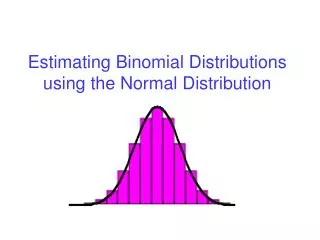
Binomial Process • The binomial process that we have described for spot rates yields after n periods a distribution of n + 1 possible spot rates. • This distribution is not normally distributed because the left-side of the distribution has a limit at zero (i.e. we generally do not have negative spot rates). • The distribution of spot rate can be converted into a distribution of logarithmic returns, gn:
Binomial Process • Note: When n = 1, there are two possible spot rates and logarithmic returns: Where: Su= uS0=S(1+u) or Sd=S(1+d) – the price can go up by u percent or down by d percent.
Binomial Process • When n = 2, there are three possible spot rates and logarithmic returns:
Binomial Process • The probability of attaining any of these rates is equal to the probability of the spot rate increasing j times in n period: pnj. In a binomial process, this probability is
Binomial Distribution • Using the binomial probabilities, the expected value and variance of the logarithmic return after one period are .022 and .0054:
Binomial Distribution • The expected value and variance of the logarithmic return after two periods are .044 and .0108:
Binomial Process • Note: The expected value and the variance are also equal to
Motivation for Binomial Model • Unable to value based on market comparables approaches • Unwilling to make assumptions about market price of risk • Heuristic model to illustrate complex concepts in continuous time models such as the Black-Scholes
Binomial Process • Let S0 denote the asset price at t=0 • Partition [0,T] into n time increments of width t • Ri=1+ri, the total return, is denoted u with probability p and d with probability (1-p) • Snj, the asset price after n periods, given j upward movements and hence n-j downward movements, Snj=ujdn-jS0
Binomial Lattice 2,2 Arc 1,1 Node 0 or 0,0 2,1 1,0 2,0 t=0 t=1 t=2
Asset Price Distribution S2,2=uuS0 =u2S0 S1,1=uS0 S2,1=udS0 =duS0 S0 S1,0=dS0 S2,0=ddS0 =d2S0 t=0 t=1 yr t=2 yr
Binomial Probabilities • Probability of observing outcome a single path to n,j:pj(1-p)n-j • The number of paths to n,j: n!/(j!(n-j)!), where n!=n*(n-1)*…*2*1 • Probability of observing n,j: (n!/(j!(n-j)!))pj(1-p)n-j
Binomial Probabilities • Consider p = 0.5, n = 3, the distribution • (3,0): 1p0(1-p)3= 0.53 = 0.125 • (3,1): ((3*2*1)/1(2*1)) p1(1-p)2 = 0.375 • (3,2): ((3*2*1)/(2*1)1) p2(1-p)1 = 0.375 • (3,3): 1p3(1-p)0 = 0.53 = 0.125 • Note there are three ways to arrive at either node (3,1) or (3,2) and the probability of any path is 0.125
Binomial Probabilities • Probability of observing n,j: • The expected asset price at n:
Bond Valuation Model • A valuation model must produce arbitrage-free values; that is, a valuation model must produce a value for each on-the-run issue that is equal to its observed market price. • There are several arbitrage-free models that can be used to value bonds with embedded options but they all follow the same principle—they generate a tree of interest rates based on some interest rate volatility assumption, they require rules for determining when any of the embedded options will be exercised, and they employ the backward induction methodology. • A valuation model involves generating an interest rate tree based on (1) benchmark interest rates, (2) an assumed interest rate model, and (3) an assumed interest rate volatility.
Valuing a Bond with an Embedded Option Using the Binomial Model
Valuing a Bond with an Embedded Option Using the Binomial Model
Valuing a Bond with an Embedded Option Using the Binomial Model • A valuation model involves generating an interest rate tree based on (1) benchmark interest rates, (2) an assumed interest rate model, and (3) an assumed interest rate volatility. • The assumed volatility of interest rates incorporates the uncertainty about future interest rates into the analysis. • The interest rate tree is constructed using a process that is similar to bootstrapping but requires an iterative procedure to determine the interest rates that will produce a value for the on-the-run issues equal to their market value. • At each node of the tree there are interest rates and these rates are effectively forward rates; thus, there is a set of forward rates for each year.
Valuing a Bond with an Embedded Option Using the Binomial Model
Valuing a Bond with an Embedded Option Using the Binomial Model • Using the interest rate tree the arbitrage-free value of any bond can be determined. • In valuing a callable bond using the interest rate tree, the cash flows at a node are modified to take into account the call option. • The value of the embedded call option is the difference between the value of an option-free bond and the value of the callable bond.
Valuing a Bond with an Embedded Option Using the Binomial Model
Valuing a Bond with an Embedded Option Using the Binomial Model
Valuing a Bond with an Embedded Option Using the Binomial Model • The volatility assumption has an important impact on the arbitrage-free value. • The option-adjusted spread is the constant spread that when added to the short rates in the binomial interest rate tree will produce a valuation for the bond (i.e., arbitrage-free value) equal to the market price of the bond. • The interpretation of the OAS, or equivalently, what the OAS is compensating an investor for, depends on what benchmark interest rates are used.
Valuing a Bond with an Embedded Option Using the Binomial Model
Valuing a Bond with an Embedded Option Using the Binomial Model
Valuing a Bond with an Embedded Option Using the Binomial Model
Valuing a Bond with an Embedded Option Using the Binomial Model


