Impedance-based techniques
Impedance-based techniques. 3-4-2014. Impedance overview. ac source. Perturb cell w/ small magnitude alternating signal & observe how system handles @ steady state Advantages: High-precision ( indef steady long term avg ) Theoretical treament


Impedance-based techniques
E N D
Presentation Transcript
Impedance-based techniques 3-4-2014
Impedance overview ac source • Perturb cell w/ small magnitude alternating signal & observe how system handles @ steady state • Advantages: • High-precision (indef steady long term avg) • Theoretical treament • Measurement over wide time (104 s to ms) or freq range (10-4 Hz to MHz) • Prototypical exp: faradaic impedance ,cell contains solution w/ both forms of redox couple so that potential of WE is fixed • Cell inserted as unknown into one arm of impedance bridge & R, C adjusted to balance • Determine values of R & C at measurement frequency • Impedance measured as Z(w) • Lock-in amplifiers, frequency response analyzers • Interpret R, C in terms of interfacial phenom • Faradaic impedance (EIS) high precision, evalheterogen charge-transfer parameters & DL structure Potentiometer to null dc voltage ac null detector cell R V C – + dc null detector I1RA= I2RB dc null detector I1Ru = I2R I1+ I2 RA Ru I1 Ru = R(RA/RB) I2 RB R
ac voltammetry • 3 electrode cell (DME ac polaragraphy) • dc mean value Edc scanned slowly w/ time plus sine component (~ 5 mV p-to-p) Eac • Measure magnitude of ac component of current and phase angle w.r.t. Eac • dc potential sets surf conc. of O and R: CO(0,t) & CR(0,t) differ from CO* and CR* diffusion layer • Steady Edc thick diffusion layer, dimensions exceed zone affected by Eac CO(0,t) & CR(0,t) look like bulk to ac signal (DPP relies on same effect) • Start w/ solution containing only one Redox form & obtain contin plots of iac amp & phase angle vs. Edc represent Faradaic impedance at continuous ratios of CO(0,t) & CR(0,t) • EIS and ac voltammetry involve v. low amp excitation sig & depend on current-overpotential relation virtually linear @ low overpotential E t
ac circuits • Rotating vector (phasor) • Consider relationship between i, e rotating at w (2pf), separated by phase angle f. e = E sinwt i = I sin (wt + f) Capacitor i = C(de/dt) q = Ce w Resistor Ė = İR i = E/XCsin (wt + p/2) XC = 1/wC p/2 ileads e Ė f 0 p İ İ Ė = –jXCİ -p/2
ac circuits: RC Y Resistor ĖR= İR f i = I sin (wt + f) Capacitor ĖC= –jXCİ R f XC = 1/wC Series Ė = ĖR+ ĖC –jXC Z Ė = İ (R – jXC) Polar Form Ė = İ Z Z = Zejf Y = Ze–jf admittance Z(w) = ZRe – jZIm |Z|2 = R2 + XC2 = (ZRe)2 + (ZIm)2 tan f= ZIm/ZRe= XC/R = 1/wRC f= 0 R only f= p/2 C only
Bode plots RC parallel Ė = İ [RXC2/(R2 + XC2) – jR2XC/(R2 + XC2)] RC series R = 100 W C = 1 mF Ė = İ (R – jXC)
Nyquist plots RC parallel RC series R = 100 W C = 1 mF Ė = İ (R – jXC) Ė = İ [RXC2/(R2 + XC2) – jR2XC/(R2 + XC2)]
Equivalent circuit of cell ic • Randles Equivalent Circuit • Frequently used • Parallel elements because iis the sum of ic, if • Cd is nearly pure C (charge stored electrostatically) • Faradaic processes cannot be rep by simple R, C which are independent of f (instead consider as general impedance Zf) Cd RW Zf ic + if if = = Rep charge transfer between electrode-electrolyte Rct Zf Zw Rs Cs • Faradaic Impedance • Simplest rep as series resistance Rs, psuedocapacitanceCs • Alternative, pure resistance Rct and Warburg Impedance (kind of resistance to mass transfer) • Components of Zf not ideal (change with f) • Equivalent Circuits • Rep cell performance at given f, not all f • Chief objective of faradaic impedance: discover f dependence of Rs, Cs apply theory to transform to chem info • Not unique
Characteristics of equiv circuit ic Cd • Measurement of total impedance includes RW and Cd • Separate Zf from RW, Cd by considering f dependence or by evalRW and Cd in separate experiment w/o redox couple RW Zf ic + if if = Zf Rs Cs • Assume Zf can be expressed as Rs, Cs in series
Description of chemical system O + ne ⇄ R (O, R soluble) E = E[i, CO(0,t), CR(0,t)] Because E is a function of 3 variables that depend on t, total differential is a combination of partial differentials by mass transfer considerations Find Initial conditions: CO(x,0) = CO*, CR(x,0) = CR* Recall from section 8.2.1: Notice the sign convention is opposite of usual
Determination of CO(0,t), CR(0,t) O + ne ⇄ R (O, R soluble) E = E[i, CO(0,t), CR(0,t)] Find Initial conditions: CO(x,0) = CO*, CR(x,0) = CR* by mass transfer considerations Recall from section 8.2.1: Recall Laplace Transform: (s) Convolution integral:
Evaluation of O + ne ⇄ R (O, R soluble) E = E[i, CO(0,t), CR(0,t)] Recall trig identity sin w(t – u) = sin wt cos wu – cos wt sin wu Can be derived from Euler identity ejx = cos x– j sin x Also recall: sin x = (ejx – e–jx)/2j, cos x = (ejx+ e–jx)/2
Evaluation of O + ne ⇄ R (O, R soluble) E = E[i, CO(0,t), CR(0,t)] Now consider time range of interest. At t=0, CO(0, t) = CO* & CR(0, t) = CR* After few cycles: steady state is reached (no net electrolysis during any full cycle) Interest is in steady state Integrals rep transition from initial cond to steady state Because u–½ appears, integrands only significant at short times Obtain steady state by letting int limits go to
Evaluation of O + ne ⇄ R (O, R soluble) E = E[i, CO(0,t), CR(0,t)] Recall: sin x = (ejx – e–jx)/2j, cos x = (ejx+ e–jx)/2 Can be derived from Euler identity ejx = cos x– j sin x
Surface concentration expressions O + ne ⇄ R (O, R soluble) E = E[i, CO(0,t), CR(0,t)]
Evaluation of Rs, Cs O + ne ⇄ R (O, R soluble) E = E[i, CO(0,t), CR(0,t)] Finding Rs, Csdepends on finding Rct, bO, bR Rct from heterogeneous charge-transfer kinetics s/w1/2 and 1/sw1/2 from mass-transfer effects Called pseudo C because energy is stored electrochemically (in rev faradaic redox reaction) rather than electrostatically (as in Cd) f dependent R ZW Pseudo C
Kinetic parameters from impedance kf O + e ⇄ R (O, R soluble) kb sine component is small, electrode’s mean potential at equilibrium use linearized i-h characteristic (see 3.4.30) to describe system (electronic current convention) k0 can be evaluated through i0 when Rs, Cs are known Rs 1/wCs R or XC Rct Slope =s w–1/2
Limiting case: reversible system, fast charge transfer i0 , Rct 0, Rs s/w1/2 ZW alone. Mass-transfer impedance (applies to any electrode reaction) minimum impedance. If kinetics are observable, Rct contributes and Zfis greater. Large concentrations reduce mass-transfer impedance Concentration ratio significantly different than one make s and Zf large Large transfer rates only achieved when concentrations are comparable (Zf minimal near E0’) Impedance measurements easiest near E0’
Limiting case: reversible system, fast charge transfer RW = s/w1/2 i0 , Rct 0, Rs s/w1/2 f < 45o 1/wCs = s/w1/2 Rct tan f= 1/wRsCs = (s/w1/2) / (Rct + s/w1/2) 0 ≤ f ≤ 45o, always a component of iac in-phase (0o) with Eac and can be measured with phase sensitive detector (lock-in amplifier) basis for discriminating against charging current in ac voltammetry |Zf| = |ZW| |Zf| > |ZW|
Electrochemical impedance spectroscopy ic • Measurement of cell characteristics includes RW and Cd • Separate Zf from RW, Cd by considering f dependence (EIS) or by evalRW and Cd in separate experiment w/o redox couple (Impedance bridge) • Randles Equivalent Circuit • Frequently used • Parallel elements because iis the sum of ic, if • Cd is nearly pure C • Faradaic processes cannot be rep by simple R, C which are independent of f (instead consider as general impedance Zf) Cd RW Zf ic + if if = Zw Zf Rs Cs = Rct EIS: study the way Z = RB – j/wCB = ZRe – jZImvaries with f Extract RW, Cd, Rs, and Cs Eliminates need for separate measurements w/o redox species Eliminates need to assume redox species has no effect on nonfaradaic impedance
Electrochemical impedance spectroscopy ic • Based on similar methods used to analyze circuits in EE practice • Developed by Sluyters and coworkers • Variation of total impedance in complex plane (Nyquist plots) Cd RW Zf ic + if if = Zf Rs Cs Measured Z is expressed as series RB + CB ZRe = RB , ZIm = 1/wCB See Section 10.1.2 Can be shown by E = ERW + ECd(ERs + ECs)/(ECd + ERs +ECs) ER = IR, EC = –j/wC A = Cd/Cs , B = wRsCd
Variation of total impedance ic Cd A = Cd/Cs , B = wRsCd RW Zf ic + if if = Zf Rs Cs Obtain chem info by plotting Zimvs. ZRe
Impedance: low-frequency limit As w 0 • Linear w/ unit slope and extrapolated line intersects ZRe axis at • Indicative of diffusion-controlled electrode process (under mass transfer control) • As f increases, Rct and Cd become more important leading to departure from ideal behavior ZIm Slope = 1 ZRe
Impedance: high-frequency limit As w Cd Cd RW Rct • Circular plot center at (RW + Rct/2, 0), r = Rct/2 • At high f, all i is ic and only impedance comes from RW • As f decreases, Cd significant ZIm • At v. low f, Cd high Z, i mostly through Rct and RW • Expect departure in low f because ZW is important there RW Zf w = 1/RctCd ZIm RW RW + Rct ZRe
Impedance: applications to real systems w = 1/RctCd ZIm RW RW + Rct ZRe Mass-transfer control Kinetic control In real systems, both regions may not be well defined depending on Rct and its relation to ZW (s). If system is kinetically slow, large Rctand only limited f region where mass transfer significant.If Rct v. small in comparison to RW and ZW over nearly all s, system is so kinetically facile that mass transfer always plays a role. w = 1/RctCd ZIm ZIm RW RW + Rct ZRe ZRe
Limits to measurable k0 by faradaic impedance • Upper limit • Rct must make sig contribution to Rs (Rct ≥ s/w1/2) • k0 ≤ (Dw/2)1/2 (assume DO=DR, CO* = CR*) • Highest practical w is determined by RuCd≤ cycle period of ac stimulus • For UME, useful measurements at w ≤ 107 s-1, with D ~ 10-5 cm2/s, k0 ≤ 7 cm/s • Think aromatic species to cation/anion radicals in aprotic solvents (k0 > 1 cm/s) • Cs ≥ Cd and Rs ≥ RW Mass-transfer control Kinetic control w = 1/RctCd ZIm RW RW + Rct ZRe i0 = FAk0C (Eqn 3.4.7) • Lower limit • Large Rct, ZW negligible • Rct cannot be so large that all i through Cd (Rct≤ 1/wCd) k0≥ RTCdw/F2C*A • For C* = 10-2 M and w = 2p x 1 Hz, T=298, Cd/A = 20 mF/cm2 k0≥ 3 x 10⁻⁶ cm/s
EIS and other applications • More complicated systems (couple homogeneous reactions, adsorbed intermediates) can also be explored with EIS • General strategy: obtain Nyquist plots and compare to theoretical models based on appropriate eqns rep rates of various processes and contributions to i(t) • May be useful to represent system by equivalent circuit (R, C, L), but not unique and cannot be easily predicted from reaction scheme • Electrode surf roughness and heterogeneity can also affect ac response (smooth, homogeneous Hg electrodes generally better than solid electrodes) • Application to variety of systems: corrosion, polymer film, semiconductor electrodes
Instrumentation • Impedance measurements made in either f domain with frequency response analyzer (FRA) or t domain using FT with a spectrum analyzer • FRA generates e(t) = D sin(wt) and adds to Edc • take care to avoid f and amplitude errors that can be introduced by the potentiostat, particularly at high f • Vi(t) to analyzer, mixed with input signal and integrated over several periods to give ZIm, ZRe • Frequency range of 10 mHz to 20 MHz • Spectrum analyzer: Echem system subjected to potential variation resultant of many frequency (pulse, white noise signal), and i(t) is recorded • Stimulus and response converted via FT to spectral rep of amp and f vs. f • Allow interpretation of experiments in which several different excitation signals applied to chem system at same time (multiplex advantage) • Responses are superimposed but FT resolves them
Additional references/further reading • Sluyters-Rehbach, Pure & Appl. Chem. 1994, 66:1831-1891. • Orazem & Tribollet, Electrochemical Impedance Spectroscopy, 2008, John Wiley & Sons: Hoboken, NJ.