Leveraging IBM Cell for High-Performance Linear Algebra Computations
The IBM Cell processor, notably used in PlayStation 3, features a PowerPC core with eight synergistic processing elements (SPEs), enabling extraordinary performance in linear algebra tasks. With a peak performance of 204.8 Gflop/s in single precision and 14.6 Gflop/s in double precision, it allows for efficient mixed-precision iterative refinement techniques for solving dense linear systems. By exploiting the capabilities of single precision for most calculations and refining with double precision, the Cell architecture can achieve significant performance gains while maintaining accuracy, especially in computationally intensive applications.


Leveraging IBM Cell for High-Performance Linear Algebra Computations
E N D
Presentation Transcript
IBM Cell for Linear Algebra Computations The Innovative Computing Laboratory University of Tennessee Knoxville Oak Ridge National Laboratory
With the hype on Cell and PS3we became interested • The PlayStation 3's CPU based on a "Cell“ processor. • Each Cell contains a Power PC processor and 8 SPEs (SPE is processing unit, SPE: SPU + DMA engine). • An SPE is a self-contained vector processor that acts independently from the others. • 4 way SIMD floating point units capable of a total of 25.6 Gflop/s @ 3.2 GHZ. • 204.8 Gflop/s peak! • The catch is that this is for 32 bit floating point; (single precision, SP). • And 64 bit floating point runs at 14.6 Gflop/s total for all 8 SPEs!! • Divide SP peak by 14; factor of 2 because of DP and 7 because of latency issues. SPE ~ 25 Gflop/s peak
Performance of single precision on conventional processors • We have the similar situation on our commodity processors. • That is, SP is 2X as fast as DP on many systems. • The Intel Pentium and AMD Opteron have SSE2: • 2 flops/cycle DP • 4 flops/cycle SP • IBM PowerPC has AltiVec: • 8 flops/cycle SP • 4 flops/cycle DP • No DP on AltiVec Single precision is faster because • Higher parallelism in SSE/vector units • Reduced data motion • Higher locality in cache
32 or 64 bit floating point precision? • A long time ago, 32 bit floating point was used. • Still used in scientific apps but limited. • Most apps use 64 bit floating point. • Accumulation of round off error: • A 10 Tflop/s computer running for 4 hours performs > 1 exaflop (1018) ops. • Ill conditioned problems: • IEEE SP exponent bits too few (8 bits, 10±38). • Critical sections need higher precision— • Sometimes need extended precision (128 bit floating point). • However, some can get by with 32 bit floating point in some parts. • Mixed precision is a possibility. • Approximate in lower precision and then refine or improve solution to high precision.
Idea goes something like this… • Exploit 32 bit floating point as much as possible— • especially for the bulk of the computation. • Correct or update the solution with selective use of 64 bit floating point to provide refined results. • Intuitively • compute a 32 bit result, • calculate a correction to 32 bit result using selected higher precision, and • perform the update of the 32 bit results with the correction using high precision.
Mixed-precision iterative refinement • Iterative refinement for dense systems, Ax = b, can work this way. L U = lu(A)SINGLEO(n3) x = L\(U\b) SINGLEO(n2) r = b – Ax DOUBLEO(n2) WHILE || r || not small enough z = L\(U\r) SINGLEO(n2) x = x + z DOUBLEO(n1) r = b – Ax DOUBLEO(n2) END
Mixed-precision iterative refinement • Iterative refinement for dense systems, Ax = b, can work this way. • Wilkinson, Moler, Stewart, and Higham provide error bound for SP floating point results when using DP fl pt. • It can be shown that, using this approach, we can compute the solution to 64-bit floating point precision. • Requires extra storage, total is 1.5 times normal. • O(n3) work is done in lower precision. • O(n2) work is done in high precision. • Problems if the matrix is ill-conditioned in sp; O(108).
Results for mixed precision iterative refinement for dense Ax = b • Single precision is faster than DP because of • higher parallelism within vector units • 4 ops/cycle (usually) instead of 2 ops/cycle • reduced data motion • 32 bit data instead of 64 bit data • higher locality in cache • More data items in cache
Results for mixed precision iterative refinement for dense Ax = b
What about the Cell? • Power PC at 3.2 GHz: • DGEMM at 5 Gflop/s. • Altivec peak at 25.6 Gflop/s— • Achieved 10 Gflop/s SGEMM. • 8 SPUs • 204.8 Gflop/s peak! • The catch is that this is for 32 bit floating point (single precision SP). • And 64 bit floating point runs at 14.6 Gflop/s total for all 8 SPEs!! • Divide SP peak by 14; factor of 2 because of DP and 7 because of latency issues.
Moving data around on the Cell 256 KB 25.6 GB/s Injection bandwidth Injection bandwidth Worst-case memory-bound operations (no reuse of data). three data movements (2 in and 1 out) with 2 ops (SAXPY) for the Cell would be 4.6 Gflop/s (25.6 GB/s*2ops/12B).
IBM Cell 3.2 GHz, Ax = b 8 SGEMM (embarrassingly parallel) 0.30 secs 3.9 secs
8.3X IBM Cell 3.2 GHz, Ax = b 8 SGEMM (embarrassingly parallel) 0.30 secs 0.47 secs 3.9 secs
Cholesky on the Cell, Ax=b, A=AT, xTAx > 0 Single precision performance Mixed precision performance using iterative refinement Method achieving 64 bit accuracy For the SPE’s standard C code and C language SIMD extensions (intrinsics) 14
Intriguing potential Exploit lower precision as much as possible Payoff in performance Faster floating point Fewer data to move Automatically switch between SP and DP to match the desired accuracy Compute solution in SP and then a correction to the solution in DP Potential for GPU, FPGA, special purpose processors What about 16 bit floating point? Use as little you can get away with and improve the accuracy Applies to sparse direct and iterative linear systems and Eigenvalue, optimization problems, where Newton’s method is used
IBM/Mercury Cell blade • From IBM or Mercury • 2 Cell chip • Each w/8 SPEs • 512 MB/Cell • ~$8K–17K • Some SW
Sony Playstation 3 cluster PS3-T • From IBM or Mercury • 2 Cell chip • Each w/8 SPEs • 512 MB/Cell • ~$8K–17K • Some SW • From WAL*MART PS3 • 1 Cell chip • w/6 SPEs • 256 MB/PS3 • $600 • Download SW • Dual boot
PE PE PE PE PE PE PE PE Cell hardware overview SIT CELL 25.6 Gflop/s 25.6 Gflop/s 25.6 Gflop/s 25.6 Gflop/s 200 GB/s PowerPC 25.6 Gflop/s 25.6 Gflop/s 25.6 Gflop/s 25.6 Gflop/s 25 GB/s 3.2 GHz 25 GB/s injection bandwidth 200 GB/s between SPEs 32 bit peak perf 8*25.6 Gflop/s 204.8 Gflop/s peak 64 bit peak perf 8*1.8 Gflop/s 14.6 Gflop/s peak 512 MB memory 512 MiB
PE PE PE PE PE PE PS3 hardware overview SIT CELL 25.6 Gflop/s Disabled/broken: Yield issues 25.6 Gflop/s 25.6 Gflop/s 200 GB/s GameOS Hypervisor PowerPC 25.6 Gflop/s 25.6 Gflop/s 25.6 Gflop/s 25 GB/s 3.2 GHz 25 GB/s injection bandwidth 200 GB/s between SPEs 32 bit peak perf 6*25.6 Gflop/s 153.6 Gflop/s peak 64 bit peak perf 6*1.8 Gflop/s 10.8 Gflop/s peak 1 Gb/s NIC 256 MiB memory 256 MiB
PlayStation 3 LU codes 6 SGEMM (embarrassingly parallel)
PlayStation 3 LU codes 6 SGEMM (embarrassingly parallel)
HPC in the living room 33 24
What's good Very cheap: ~4$ per Gflop/s (with 32 bit floating point theoretical peak). Fast local computations between SPEs. Perfect overlap between communications and computations is possible (Open-MPI running): PPE does communication via MPI. SPEs do computation via SGEMMs. What's bad Gigabit network card. 1 Gb/s is too little for such computational power (150 Gflop/s per node). Linux can only run on top of GameOS (hypervisor): Extremely high network access latencies (120 usec). Low bandwidth (600 Mb/s). Only 256 MB local memory. Only 6 SPEs. Matrix Multiple on a 4 Node PlayStation3 Cluster Gold: Computation: 8 msBlue: Communication: 20 ms 33
Users guide for SC on PS3 • SCOP3: A Rough Guide to Scientific Computing on the PlayStation 3 • See web page for detailswww.netlib.org/utk/people/JackDongarra/PAPERS/scop3.pdf 33
Conclusions • For the last decade or more, the research investment strategy has been overwhelmingly biased in favor of hardware. • This strategy needs to be rebalanced—barriers to progress are increasingly on the software side. • Moreover, the return on investment is more favorable to software. • Hardware has a half-life measured in years, while software has a half-life measured in decades. • High performance ecosystem is out of balance: • hardware, OS, compilers, software, algorithms, applications— • no Moore’s Law for software, algorithms and applications.
Collaborators / support Alfredo Buttari, UTK Julien Langou, UColorado Julie Langou, UTK Piotr Luszczek, MathWorks Jakub Kurzak, UTK Stan Tomov, UTK 33