Download
1 / 49
490 likes | 542 Views
Explore the world of image warping and computational photography with Derek Hoiem from the University of Illinois. Learn about gradient domain editing, reconstruction from gradients, and non-photorealistic rendering. Dive into advanced projects and take-home questions to enhance your skills.

E N D
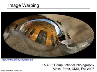
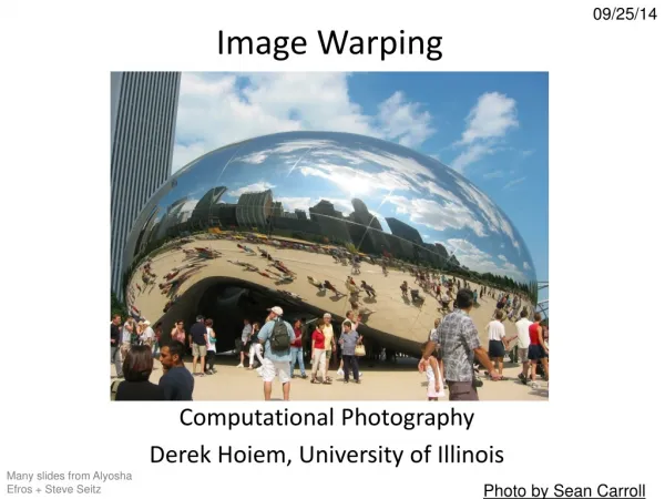
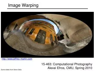
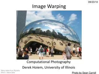
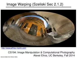
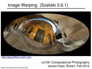
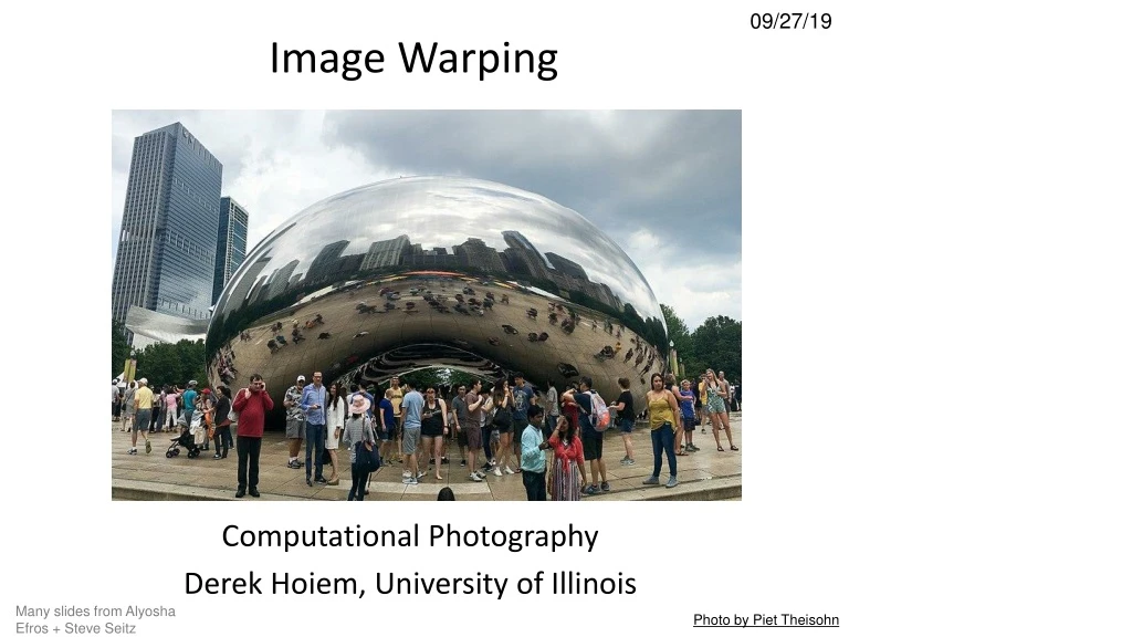
09/27/19 Image Warping Computational Photography Derek Hoiem, University of Illinois Many slides from Alyosha Efros + Steve Seitz Photo by Piet Theisohn
Reminder: Proj 2 due Tues • Much more difficult than project 1 – get started asap if not already • Must compute SSD cost for every pixel (slow but not horribly slow using filtering method; see tips at end of project page) • Learn how to debug visual algorithms: imshow, plot, breakpoints are helpful • Debugging suggestion: For “quilt_simple”, first set upper-left patch to be upper-left patch in source and iteratively find minimum cost patch and overlay --- should reproduce original source image, at least for part of the output
Review from last class: Gradient Domain Editing General concept: Solve for pixels of new image that satisfy constraints on the gradient and the intensity • Constraints can be from one image (for filtering) or more (for blending)
Project 3: Reconstruction from Gradients • Preserve x-y gradients • Preserve intensity of one pixel Source pixels: s Variable pixels: v • minimize (v(x+1,y)-v(x,y) - (s(x+1,y)-s(x,y))^2 • minimize (v(x,y+1)-v(x,y) - (s(x,y+1)-s(x,y))^2 • minimize (v(1,1)-s(1,1))^2
Project 3 (extra): NPR • Preserve gradients on edges • e.g., get canny edges with edge(im, ‘canny’) • Reduce gradients not on edges • Preserve original intensity Perez et al. 2003
Colorization using optimization • Minimize squared color difference, weighted by intensity similarity • Solve with sparse linear system of equations • Solve for uv channels (in Luv space) such that similar intensities have similar colors http://www.cs.huji.ac.il/~yweiss/Colorization/
Gradient-domain editing Many image processing applications can be thought of as trying to manipulate gradients or intensities: • Contrast enhancement • Denoising • Poisson blending • HDR to RGB • Color to Gray • Recoloring • Texture transfer See Perez et al. 2003 for many examples
Gradient-domain processing Saliency-based Sharpening
Gradient-domain processing Non-photorealistic rendering
Take-home questions 1) I am trying to blend this bear into this pool. What problems will I have if I use: • Alpha compositing with feathering • Laplacian pyramid blending • Poisson editing? Poisson Editing Lap. Pyramid
Take-home questions 2) How would you make a sharpening filter using gradient domain processing? What are the constraints on the gradients and the intensities?
Next two classes: warping and morphing • This class • Global coordinate transformations • Image alignment • Next class • Interpolation and texture mapping • Meshes and triangulation • Shape morphing
Photo stitching: projective alignment Find corresponding points in two images Solve for transformation that aligns the images
Capturing light fields Estimate light via projection from spherical surface onto image
Morphing Blend from one object to other with a series of local transformations
Image Transformations f f f T T x x x f x image filtering: change range of image g(x) = T(f(x)) image warping: change domain of image g(x) = f(T(x))
Image Transformations T T image filtering: change range of image g(x) = T(f(x)) f g image warping: change domain of image g(x) = f(T(x)) f g
Parametric (global) warping T Transformation T is a coordinate-changing machine: p’ = T(p) What does it mean that T is global? • Is the same for any point p • can be described by just a few numbers (parameters) For linear transformations, we can represent T as a matrix p’ = Mp p = (x,y) p’ = (x’,y’)
Parametric (global) warping Examples of parametric warps: aspect rotation translation perspective cylindrical affine
Scaling • Scaling a coordinate means multiplying each of its components by a scalar • Uniform scaling means this scalar is the same for all components: 2
Scaling X 2,Y 0.5 • Non-uniform scaling: different scalars per component:
Scaling • Scaling operation: • Or, in matrix form: scaling matrix S What is the transformation from (x’, y’) to (x, y)?
2-D Rotation (x’, y’) (x, y) x’ = x cos() - y sin() y’ = x sin() + y cos()
2-D Rotation (x’, y’) (x, y) Polar coordinates… x = r cos (f) y = r sin (f) x’ = r cos (f + ) y’ = r sin (f + ) Trig Identity… x’ = r cos(f) cos() – r sin(f) sin() y’ = r sin(f) cos() + r cos(f) sin() Substitute… x’ = x cos() - y sin() y’ = x sin() + y cos() f
2-D Rotation This is easy to capture in matrix form: Even though sin(q) and cos(q) are nonlinear functions of q, • x’ is a linear combination of x and y • y’ is a linear combination of x and y What is the inverse transformation? • Rotation by –q • For rotation matrices R
2x2 Matrices What types of transformations can be represented with a 2x2 matrix? 2D Identity? 2D Scale around (0,0)?
2x2 Matrices What types of transformations can be represented with a 2x2 matrix? 2D Rotate around (0,0)? 2D Shear?
2x2 Matrices What types of transformations can be represented with a 2x2 matrix? 2D Mirror about Y axis? 2D Mirror over (0,0)?
2x2 Matrices What types of transformations can be represented with a 2x2 matrix? 2D Translation? NO!
All 2D Linear Transformations • Linear transformations are combinations of … • Scale, • Rotation, • Shear, and • Mirror • Properties of linear transformations: • Origin maps to origin • Lines map to lines • Parallel lines remain parallel • Ratios are preserved • Closed under composition
Homogeneous Coordinates Q: How can we represent translation in matrix form?
Homogeneous Coordinates Homogeneous coordinates represent coordinates in 2 dimensions with a 3-vector
Homogeneous Coordinates y 2 (2,1,1) or (4,2,2) or (6,3,3) 1 x 2 1 2D Points Homogeneous Coordinates • Append 1 to every 2D point: (x y) (x y 1) Homogeneous coordinates 2D Points • Divide by third coordinate (x y w) (x/w y/w) Special properties • Scale invariant: (x y w) = k * (x y w) • (x, y, 0) represents a point at infinity • (0, 0, 0) is not allowed Scale Invariance
Homogeneous Coordinates Q: How can we represent translation in matrix form? A: Using the rightmost column:
Translation Example tx = 2ty= 1
Basic 2D transformations as 3x3 matrices Translate Scale Rotate Shear
Matrix Composition Transformations can be combined by matrix multiplication p’ = T(tx,ty) R(Q) S(sx,sy) p Does the order of multiplication matter?
Affine Transformations • Affine transformations are combinations of • Linear transformations, and • Translations • Properties of affine transformations: • Origin does not necessarily map to origin • Lines map to lines • Parallel lines remain parallel • Ratios are preserved • Closed under composition
Projective Transformations • Projective transformations are combos of • Affine transformations, and • Projective warps • Properties of projective transformations: • Origin does not necessarily map to origin • Lines map to lines • Parallel lines do not necessarily remain parallel • Ratios are not preserved • Closed under composition • Models change of basis • Projective matrix is defined up to a scale (8 DOF)
2D image transformations • These transformations are a nested set of groups • Closed under composition and inverse is a member
Recovering Transformations What if we know f and g and want to recover the transform T? • willing to let user provide correspondences • How many do we need? ? T(x,y) y y’ x x’ f(x,y) g(x’,y’)
Translation: # correspondences? • How many Degrees of Freedom? • How many correspondences needed for translation? • What is the transformation matrix? ? T(x,y) y y’ x x’
Euclidean: # correspondences? • How many DOF? • How many correspondences needed for translation+rotation? ? T(x,y) y y’ x x’
Affine: # correspondences? • How many DOF? • How many correspondences needed for affine? ? T(x,y) y y’ x x’
Affine transformation estimation • Math • Matlab demo
Projective: # correspondences? • How many DOF? • How many correspondences needed for projective? ? T(x,y) y y’ x x’
Take-home Question 1) Suppose we have two triangles: ABC and A’B’C’. What transformation will map A to A’, B to B’, and C to C’? How can we get the parameters? B’ B ? T(x,y) C’ A C A’ Source Destination
Take-home Question 2) Show that distance ratios along a line are preserved under 2d linear transformations. o o (x3,y3) (x’3,y’3) o o o o (x’2,y’2) (x2,y2) p‘1=(x’1,y’1) p1=(x1,y1) Hint: Write down x2 in terms of x1 and x3, given that the three points are co-linear