Download
1 / 16
160 likes | 314 Views
Numerical Model of Solar Eruption on 1998 May 2. Ilia Roussev, Igor Sokolov & Tamas Gombosi University of Michigan Terry Forbes & Marty Lee University of New Hampshire. NOAA AR8210: Summary of Observations.

E N D
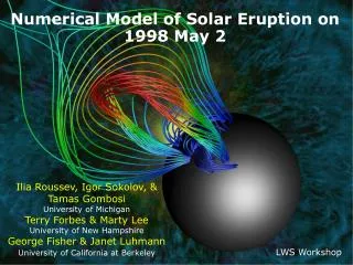
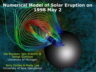
Numerical Model of Solar Eruption on 1998 May 2 Ilia Roussev, Igor Sokolov & Tamas Gombosi University of Michigan Terry Forbes & Marty Lee University of New Hampshire
NOAA AR8210: Summary of Observations • Series of intense flares and CMEs, including homologous events, occurred in NOAA AR8210 from April through May of 1998; • CME event we consider took place on 1998 May 2 near disk center (S15o,W15o), and CME speed inferred from observations by LASCO was in excess of 1,040 km/s; • X1.1/3B flare occurred in NOAA AR8210 at 13:42 UT, which was associated with SEP event observed by NOAA GOES-9 satellite. Ground-level event was observed by CLIMAX neutron monitor; • Total magnetic energy estimated from EIT dimming volume during eruption was 2.0x1031 ergs; • AR8210 constituted classic delta-spot configuration; main spot in AR8210 had large negative polarity, and it appeared to rotate relative to surrounding magnetic structures; • Sequence of cancellation events took place between central spot and newly emerging magnetic features of opposite polarity in surrounding region; • Flux emergence and subsequent cancellation may have been responsible for triggering solar eruption!
Bibliography on AR8210 • NOAA AR8210 was studied extensivelyaround the Globe: from Alabama, California, Hawaii, and Montana in USA, across France & Germany in Europe, through the Great Wall, to China and Japan: Wang et al. (2002, ApJ, 572); Xia et al. (2002, Chinese A&A, 26); Sterling et al. (2001, ApJ, 561); Sterling et al. (2001, ApJ, 560); Pohjolainen et al. (2001, ApJ, 556); Warmuth et al. (2000, Sol. Phys., 194). • Roussev et al. (2004, ApJ, in press) presented numerical model of solar eruption on 1998 May 2.
(from Fisher et al. 2003) Local Correlation Tracking shows shear along neutral line! Reconstruction of Surface Flows Surface flow pattern of NOAA AR8210 (MURI/SHINE event: 1998 May 1-2)
Field Structure of NOAA AR8210 on 1998 May 1 (Mees Observatory) Observations of Field Evolution MDI movie showing time-evolution of NOAA AR8210 from 30oE to 30oW (from Sam Coradetti )
Numerical Model • We start with magnetic field obtained using Potential Field Source Surface Method. • Spherical harmonic coefficients are obtained from magnetogram data of Wilcox Solar Observatory. They are derived using Carrington maps for rotations 1935 and 1936. • We use empirical model presented by Roussev et al. (2003, ApJ, 595, L57) to evolve MHD solution to steady-state solar wind, with helmet-type streamer belt around Sun. • Once steady-state is achieved, we begin inducing transverse motions at solar surface localized to AR8210. • These boundary motions resemble following observational facts: • Sunspot rotation;and • Magnetic flux cancellation. • Numerical techniques similar to ours have been used in past to create flux ropes and initiate CMEs in idealized, bi-polar (Inhester et al. 1992; Amari et al. 1999, 2000, 2003), and multi-polar (Antiochos et al. 1999) type magnetic configurations;
Result: flux rope erupts! + How to Achieve Solar Eruption? • 3D simulations of erupting flux ropes (after Amari et al. 1999, 2000) Numerical recipe to create flux ropes: 1. Apply shear motions along polarity inversion line: • Evolve potential field to non-potential, force-free field; • Build energy in sheared field needed for solar eruption. 2. Apply converging motions towards polarity inversion line: • Field lines begin to reconnect and form flux rope; • Some energy (~8-17%) built during shearing phase is converted into heat and kinetic energy of plasma bulk motions.
Converging motionsresemble effects of magnetic flux cancellation Vortex motionsrepresent sunspot rotation Boundary Motions Map of radial magnetic field strength (in units of Gauss), and structure of boundary motions near polarity inversion line (dashed line in green) of AR810.
Numerical Setup & Performance • Computations performed in cubic box: {-30<x<10,-20<y<20,-20<z<20}RS . • Non-uniform Cartesian block-adaptive grid: • 9 levels of body-focused refinement with finest cells near Sun; • 2 additional levels of refinement in vicinity of AR8210 to better resolve boundary motions; • Total number of cells of 3,116,352; • smallest cell-size of 4.883x10⁻³RS; • largest cells-size of 2.5RS; • Numerical resolution increased along direction of flux rope propagation by adding 25% more cells (total of 3,890,944) via 4 levels of refinement (finest cells of size 0.156RS=109,200km). • Boundary conditions describe: • “Impenetrable” and highly conducting spherical inner body at R=RS; • All velocity components at surface fixed at zero as MHD solution evolves towards steady-state (solar rotation not applied); • Small positive mass flow through inner boundary is allowed to balance mass loss by solar wind; • Line-tied boundary condition used for magnetic field; field remains frozen to plasma, except in regions where flux cancellation occurs; • Zero-gradient condition applied to all variables at outer boundaries. • Performance: • CPU power: 15 dual AMD Athlon 1900XP nodes, 1,024MB RAM per node; • Simulated time: 7.12hrs; • Running time: 441hrs CPU time; - far from doing real time simulations at present!
View of Eruption at t=1hour Solid lines are magnetic field lines; false color code shows magnitude of current density. Flow speed is shown on translucent plane given by y=0. Values in excess of 1,000 km/s are blanked and shown in light grey. Inner sphere corresponds to R=RS; color code shows distribution of radial magnetic field. Regions with radial field strength greater than 3 Gauss are blanked.
Trajectories & Speed Curves Trajectory curves of flux rope and shock (blue curves) in plane y=0. Radial velocities of rope and shock are shown by corresponding black curves.
Shock Evolution Time-evolution of shock compression ratio and fast-wave Mach number (dashed red curve).
Summary of Results Model: • Our model incorporates magnetogram data from Wilcox Solar Observatory and loss-of-equilibrium mechanism to initiate solar eruption. • Eruption is achieved by slowly evolving boundary conditions for magnetic field to account for: • Sunspot rotation;and • Flux emergence. Results: • Excess magnetic energy built in sheared field prior to eruption is 1.311x1031 ergs; • Flux rope ejected during eruption achieves maximum speed in excess of 1,040 km/s — in good agreement with observations; • CME-driven shock reaches fast-mode Mach number in excess of 4 and compression ratio greater than 3 at distance of 4 RS from solar surface. Conclusion: • CME-driven shock can develop close to Sun sufficiently strong to account for energetic solar protons up to 10 GeV! - more on this from Igor
Future Work • Use high-resolution vector magnetograph data and more realistic boundary motions to achieve eruption. • Apply similar numerical procedure to simulate other MURI & SHINE events.