Download
1 / 36
360 likes | 484 Views
Division on Impacts on Agriculture, Forest and Natural Ecosystems (IAFENT). Responsible Prof. Riccardo Valentini. Lecce, 25 Marzo 2009. IAFENT ACTIVITIES. The research activity of the IAFENT Division is divided into three MacroActivities (MA):

E N D
Division on Impacts on Agriculture, Forest and Natural Ecosystems (IAFENT) Responsible Prof. Riccardo Valentini Lecce, 25 Marzo 2009
IAFENT ACTIVITIES The research activity of the IAFENT Division is divided into three MacroActivities (MA): MA1 - Impacts on land use, agriculture and natural ecosystems MA2 - Climate change, carbon cycle and desertification MA3 - Impacts on crop water requirements and water resources management in agriculture
IAFENT MA2 SUB- ACTIVITIES The activities of MA2 can be divided into three sub-activities: A2.1 - Evaluation of carbon sources and sinks allocation and feedbacks between the carbon cycle and the climatic system A2.2 - Climate changes’ impacts on forest and natural ecosystems A2.3 - Desertification risk evaluation through integration of biophysical parameters and socio-economic indicators
A2.1 LPJ parameter optimization LPJ • LPJ is a process-based model representing key ecosystem processes governing terrestrial biogeochemistry and biogeography • LPJ simulates the water and carbon exchange between biosphere and atmosphere by means of a given set of parameters and input variables • Vegetation is described in terms of the Fractional Percentage Coverage (FPC) of 9 different Plant Functional Types (PFTs) that are able to compete for space and resources • Seven PTFs are woody (three temperate, two tropical and two boreal) and two herbaceous
A2.1 LPJ parameter optimization LPJ-DA (Data Assimilation) model version Data assimilation techniques are generally used to find an optimal combination of parameter values that minimise a cost-function which describes the misfits between observation and model results
A2.1 LPJ parameter optimization - The most important parameter controlling a given variable have been computed by means the Partial CorrelationCoefficient (PCC) - On the basis of PCC results and the knowledge of the model formulation, we chose to constrain 12 parameters controlling directly or indirectly gross primary production and evapotranspiration: 5 of these are used to compute photosynthesis, 3 to compute water stress and water balance and the other 4 are specific PFT parameters - Optimization was made via a Monte Carlo Markov chain (MCMC) procedure, showing the best performances in dealing with non-linear problems.
A2.1 LPJ parameter optimization • Daily values of ET and GPP, measured with EC technique in 10 different CarboeuropeIP sites are compared with modeled data. • The study sites were chosen in order to represent all European forest types
A2.1 LPJ parameter optimization By using separately or averaged observed data for the years 2000-2001-2002, different optimization schemes have been tested. The best resulted the one in which Data assimilation is made year by year; the optimal values are estimated with the means computed using only the 2nd-half of n points for each sequence Tmin = 0.05 Tmean = 2.27 GPP: Gross Primary Production ET: Evapotranspiration NEE: Net Ecosystem Exchange (NEE) TER: Total Ecosystem Respiration (TER).
A2.1 LPJ parameter optimization • Some parameters are close to priors • Uncertainty reduction (except gm) Prior and posterior parameter values and uncertainties for the normalized parameters. The boxes show the prior parameter values and their associated standard deviations; circle indicates optimized-posterior values and the error bars denote the standard deviation associated to the posterior parameters.
A2.1 LPJ parameter optimization The final-optimized parameters were then used to simulate water and carbon fluxes by LPJ for the year 2003 with the aim of methodology validation. Results show a decreasing both for R2 and for RMSE between observed and simulated data. Further 2003 data wereusedtoevaluae the LPJ-DA performance in simulatingvegetationresponsetoextremeevents (e.gheatwaveduring the summer 2003). European-wide anomaly of GPP during the summer 2003. The figure represents the difference, averaged over JJA, between prior and posterior, for the summer 2003. Relative increments between prior and posterior (final-optimized) squared correlation coefficients (R2) and root mean squared error (RMSE).
A2.1 LPJ parameter optimization CONCLUSIONS ON DATA ASSIMILATION • This study has demonstrated how data assimilation provides a powerful tool for analyzing ecosystem processes and it might help to improve our understanding about carbon and water exchange between land ecosystem and atmosphere • The optimization helps to retrieve a better knowledge about some LPJ ecophysiological parameters and uncertainties • Final-optimized values are very close for almost all parameters to the prior values
A2.1 Feedbacks of vegetation on climate LPJ è stato usato per investigare come i cambiamenti della copertura del suolo possono influire sul clima, utilizzando il modello RegCM3. Sono state fatte tre simulazioni: Controllo (CTL): utilizzando la copertura attuale Deforestazione (DEF): sostituzione delle foreste con le coltivazioni, soprattutto nell’Europa dell’Est Afforestazione (AFF): sostituzione delle coltivazioni con le foreste, in particolare in Europa Centrale. RegCM-Test: Resolution: 30 Km Time Step: 100 s Boundary Conditions: u, v, T, q, SST (6 hourly) Vertical levels: 18 sigma levels Simulation length: 1981-2000 Grid points: 150x160 in lon-lat direction respectively
A2.1 Feedbacks of vegetation on climate • CTL present vegetation cover: the surface vegetation and landuse types are obtained from satellite information and interpolated into model grid; at each grid element is assigned a dominant type of land cover
A2.1 Feedbacks of vegetation on climate • CAUSES OF DEFORESTATION IN EUROPE • Land use changes (e.g. Poland) • Air pollution • Drought effect • Overgrazing • DEF: starting from GLCC dataset, we substituted all the forests and the trees below 800 meters with crops
A2.1 Feedbacks of vegetation on climate • CAUSES OF AFFORESTATION • Poor quality of soil • Difficult access of farm • Steep slopes • High labor requirements • Farmers’ age and health • AFF: considers a plausible evolution to a spontaneous afforestation situation caused by abandonment of crops and fields which lead to a natural recapture by forests of abandonment of arable land
A2.1 Feedbacks of vegetation on climate CONCLUSIONS ON VEGETATION-CLIMATE FEEDBACKS • The simulations reveal a substantial thermodynamically and dynamically impact of vegetation on climate • Also in regions not directly affected by LCC have been found significant changes in temperature • The effects of the LCC may be in the same direction as those from increasing GHG forcing • Necessity to adopt an improved and fully dynamic vegetation in GCMs and RCMs to take into account vegetation-climate feedbacks
A2.1 ORCHIDEE forcing downscaling The ORCHIDEE model was used to evaluate the importance of the downscaling of the climate forcings to run the model at finer spatial resolution and do not miss information over coastal areas. We compared 3 simulations: a) input at 0.5x0.5° and monthly time step; b) 30 km of resolution and hourly time step; c) 10 km of resolution at and hourly time step. a) b) c)
LAND USE CHANGE (LUC) modeling IAFENT MA2 SUB- ACTIVITIES The activities of MA2 can be divided into three sub-activities: A2.1 - Evaluation of carbon sources and sinks allocation and feedbacks between the carbon cycle and the climatic system A2.2 - Climate changes’ impacts on forest and natural ecosystems A2.3 - Desertification risk evaluation through integration of biophysical parameters and socio-economic indicators LAND USE CHANGES
LAND USE CHANGE (LUC) modeling CMCC framework CLIMATE SCENARIOS (ANS) SOCIO-ECONOMICS SCENARIOS (CIP) LAND USE SCENARIOS (IAFENT) Impacts and Modifications (IAFENT, SCO) Resposes: Prevention, Mitigation Adaptation
DIAGNOSTIC APPROACH PROGNOSTIC APPROACH LAND USE CHANGE (LUC) modeling ANALYSIS OF CHANGES PAST/RECENT LAND USE ACTUAL LAND USE VALIDATION CALIBRATION MODELS ACTUAL LAND USE SIMULATION FUTURE LAND USE SIMULATION
LAND USE CHANGE (LUC) modeling Study area: Italy Diagnostic Approach: trend analysis Fifties-Sixties Land use map CNR-TCI Scale 1:200000 1990 Corine Land Cover Scale 1:100000 2000 Corine Land Cover Scale 1:25000
LAND USE CHANGE (LUC) modeling Prognostic approach: future simulations The CLUES model approach (Verburg et al., 2002) was chosen as it is a good compromise among the spatial scales, the temporal scales and the human influence it is able to take into account. Agarwal et al., 2001 • Spatially explicit • Simple and GIS-based • Different spatial scales • Every type of land use • Not constrained by specific input data • Not constrained by a given time step • Not constrained by limited study areas
LAND USE CHANGE (LUC) modeling CLUES modification • Introduction of a more reliable algorithm to calculate area on lat/long grid, more appropriate over continental scales. • the grid can also consider different fraction of land use inside each pixel, more appropriate to work at coarser resolutions. • The logistic regression among input driving factors and binary maps of presence/absence of a given land use is performed at each time step, in order to account for likely adaptation. • We introduced a more objective criterion to evaluate the effects of neighboring land use on the land use changes in a given cell.
LAND USE CHANGE (LUC) modeling Simulation Spatial resolution 500 m Simulation from 2000 to 2100 Land Use classes used in the simulation
LAND USE CHANGE (LUC) modeling Driving factors Firstly, 24 driving factors were chosen as considered influencing the land use. Elevations (digital elevation model IGMI at 20 m) Slope (calculated from 1) Aspect (calculated from 1) Soil carbon content (European Soil Database at 1 km) Soil clay content (European Soil Database at 1 km) Soil silt content(European Soil Database at 1 km) Soil sand content(European Soil Database at 1 km) Soil pH (European Soil Database at 1 km) Soil density (European Soil Database at 1 km) Soil depth (European Soil Database at 1 km) Field capacity (European Soil Database at 1 km) Population density (ISTAT, municipality scale) Labor force in agriculture (ISTAT, provincial scale) Labor force in commerce (ISTAT, local system work scale) Labor force in industry and services (ISTAT, local system work scale) Labor force in institutions (ISTAT, local system work scale) Annual mean precipitation (MARS-STAT, 50 km) Annual mean temperature (MARS-STAT, 50 km) Distance from road (road database) Distance from rivers (river network database) Distance from sea (coastal boundary database) Distance from cities (from Corine Land Cover database) Topographic index (calculated from 1) Water deficit index (calculated from 17, 18, 12 and EUROPEAN SOIL DATABASE) For each of continuous variables, the Kolmogorov-Smirnov test was performed to verify the normality of distribution Then the Spearman test was carried out to determine the non-correlation among parameters
LAND USE CHANGE (LUC) modeling LogisticRegression Driving factors Binary maps: existence (1) or not (0) for each land use FINAL DRIVING FACTORS Elevations Slope Aspect Soil carbon content Soil clay content Soil silt content Soil sand content Soil pH Soil density Soil depth Filed capacity Population density Labor force in agriculture Labor force in commerce Labor force in industry and services Labor force in institutions Annual mean precipitation Annual mean temperature Distances from the cities Topographic index Influencing factor βcomputation Calcolo dei fattori di influenza relativa perché i fattori predisponenti hanno diverse scale ed unità di misura
LAND USE CHANGE (LUC) modeling For each land use inversion of the logistic regression βfactors Driving factors Initial dicothomic map about the presence/absence of land use Pil (0-1) for each map unit (pixel) Comparison
LAND USE CHANGE (LUC) modeling Regression model accuracy For each Pil[0,1] ROC (Receiving Operating Characteristics) AREA BELOW THE CURVE =0.5 random =1 perfect It is possible to test the regression model performances considering different driving factors true positive rate (TPR) or sensitivity TPR = TP / P = TP / (TP + FN) false alarm rate (FPR) FPR = FP / N = FP / (FP + TN)
LAND USE CHANGE (LUC) modeling distance/enrichment effects among land uses in neighboring We included in the model a distance/enrichment factor (Santini et al., in prep.) avoiding to chose subjectively the distance into which calculating such factor as in (Verburg et al., 2004)
LAND USE CHANGE (LUC) modeling ELASTICITY FACTOR FUTURE LAND USE DEMAND Demands are in ha, “c” indicates the central demographic hypothesis (slight population increase) while “h” the high demographic hypothesis (strong population increase) Elasticity factors computed for mean and high impacts demands
LAND USE CHANGE (LUC) modeling 16 simulations c: central demographic hypothesis h: high demographic hypothesis a2: climate scenario a2 b2: climate scenario b2 v: vicinity/enrichment nv: no vicinity/enrichment p: protected areas np: no protected areas
LAND USE CHANGE (LUC) modeling Es. Results c_a2_nv Both for A2 and B2 climate scenarios the largest changes interest the centre of Italy (about 20%) whereas the smallest ones the north (about 18%). Anyway in the A2 scenarios changes are stronger.
LAND USE CHANGE (LUC) modeling Simulation results have been analyzed in terms of landscape fragmentation due to land use changes, using appropriate patch and landscape indices PR: PATCH RICHNESS (number of classes) SHDI: SHANNON’S DIVERSITY INDEX SIDI: SIMPSON’S DIVERSITY INDEX MSIDI: MODIFIED SIMPSON’S DIVERSITY INDEX SHEI: SHANNON’S EVENNESS INDEX SIEI: SIMPSON’S EVENNESS INDEX MSIEI: MODIFIED SIMPSON’S EVENNESS INDEX AI: AGGREGATION INDEX … Analyzing patch metric we obtained that classes of artificial land use have a behaviour differing from the one of natural or semi-natural areas 2000 c_a2_nv c_b2_nv e.g. Radius of Gyration (m)
Water Resource Index There are many drought indices (e.g., Standardize Precipitation Index) used as indicators of water resources in terms of natural recharge, but not able to represent the water reserve as they do not take into account the groundwater balance, the land use etc. Recently a Groundwater Resource Index (Mendicino et al., 2008) has been developed that considers the soil component. But in order to perform a most complete evaluation of water resources it is necessary to account for human, agricultural and industrial consumption strictly dependent from climate and land use changes. WRI = (EI-HC) Actual - Climate data MARS-STAT decade 1996-2005 - Lithological maps of Italy - Population density ISTAT • Scenarios • Climate scenario for the decades 2071-2080, 2081- 2090, 2091-2100 • - Lithological maps of Italy • - Demographic prediction ISTAT up to 2051
Future directions … Land use change model validation for the period from 1950 to 2000 (in progress) High resolutionland use change model validation (hydrographic basin scale) usingland use maps for 1800 (pre-industrial age), 1878, 1939, 1980, 2000 (in progress) Highresolution Climate scenarios CMCC (ANS division) + land use changes scenarios Desertification risk evaluation and scenarios Focusing on water resources (human, agriculture, industry, energy use) Socio-economic (CIP division) and land use change model coupling (Mediterranean Europe) Input to carbon model (ANS division) Forest type habitat migration according to forest spreading or reduction due to land use changes.
Pubblications • Magnani F. et al., co-author R. Valentini. 2008. Ecologically implausible carbon response? Reply.Nature, 451(7180): E3-E4 • - Vuichard N. et al., co-author R. Valentini. 2008. Carbon sequestration due to the abandonment of agriculture in former USSR since 1990Global Biogeochemical Cycles, 22( GB4018): doi:10.1029/2008GB003212. • - Wohlfahrt GA. et al., co-author R. Valentini. 2008. Biotic, Abiotic, and Management Controls on the Net Ecosystem CO2 Exchange of European Mountain Grassland Ecosystems. Ecosystems ,11: 1338–1351 • - Ciais P. et al., co-author R. Valentini. 2008. Carbon accumulation in European forests Nature Geosciences, 1(7): 425-4 • - Dolman A.J., A. Freibauer and R. Valentini. 2008. The continental scale greenhouse gas balance of Europe Springer, New York, 2008 • - Papale D. et al., 2008. ASPIS, A Flexible Multispectral System for Airborne Remote Sensing Environmental ApplicationsSensors (8), 3240-3256. • - Richardson A.D. et al., co-author D.Papale. 2008. Statistical properties of random CO2 flux measurement uncertainty inferred from model residuals. Agricultural and Forest Meteorology, (148), 38-50 2008 • - Göckede M. et al., co-authors D.Papale, R. Valentini. 2008. Quality control of CarboEurope flux data - Part 1: Coupling footprint analyses with flux data quality assessment to evaluate sites in forest ecosystem. Biogeosciences (5), 433-450. • - Carvalhais N. et al., co-authors D. Papale, R. Valentini. 2008. Implications of the carbon cycle steady state assumption for biogeochemical modeling performance and inverse parameter retrieval. Global Biogeochemical Cycles, (22), GB2007 • - Vetter M. et al., co-author D.Papale. 2008. Analyzing the causes and spatial pattern of the European 2003 carbon flux anomaly using seven models. Biogeosciences, (5), 561-583. • - Desai A.R. et al., co-author D.Papale, 2008. Cross-site evaluation of eddy covariance GPP and RE decomposition techniques. Agricultural and Forest Meteorology, (148), 821-838. • - Lasslop G. et al., co-author D.Papale. 2008. Influences of observation errors in eddy flux data on inverse model parameter estimation. Biogeosciences (5), 1311-1324. • Jung M. et al., co-author D. Papale. 2008. Diagnostic assessment of European gross prige mary production. Global Change Biology (14), 2349-2364. • Garbulsky M.F. et al., co-author D. Papale. 2008. Remote estimation of carbon dioxide uptake by a Mediterranean forest. Global Change Biology (14) 2860-2867. • Claus Beier et al., co-authors Duce P. and Spano D. Carbon and nitrogen balances for 6 shrublands across Europe. Global Biogeochemical Cycles (accepted) • Prieto P. Et al., co-authors Cesaraccio C., Pellizzaro G., and Sirca C. Changes in the onset of shrubland species spring growth in response to anexperimental warming along a north-south gradient in Europe. Global Ecologyand Biogeography (accepted). • M.J. Calejo, N. Lamaddalena, J.L. Teixeira, L.S. Pereira. 2008. Performance analysis of pressurized irrigation systems operating on demand using flow-driven simulation modelling. Journal of Agricultural Water Management. n. (95) 2008, pp 154-162.