Download

1 / 33
330 likes | 480 Views
One-way ANOVA. Motivating Example Analysis of Variance Model & Assumptions Data Estimates of the Model Analysis of Variance Multiple Comparisons Checking Assumptions One-way ANOVA Transformations. Motivating Example: Treating Anorexia Nervosa. Analysis of Variance.

E N D
One-way ANOVA • Motivating Example • Analysis of Variance • Model & Assumptions • Data Estimates of the Model • Analysis of Variance • Multiple Comparisons • Checking Assumptions • One-way ANOVA Transformations
Analysis of Variance • Analysis of Variance is a widely used statistical technique that partitions the total variability in our data into components of variability that are used to test hypotheses. • In One-way ANOVA, we wish to test the hypothesis: H0: 1= 2= = k against: Ha:Not all population means are the same
= m + a + e x ij i ij Model & Assumptions • The model for the observed response is given by: • We assume that the errors are normally distributed with constant variance. • This implies that the populations being sampled are also normally distributed with equal variances!
Analysis of Variance • In ANOVA, we compare the between-group variation with the within-group variation to assess whether there is a difference in the population means. • Thus by comparing these two measures of variance (spread) with one another, we are able to detect if there are true differences among the underlying group population means.
Analysis of Variance • If the variation between the sample means is large, relative to the variation within the samples, then we would be likely to detect significant differences among the sample means.
Between Group Variation is Large Compared to Within Group Variation Here we would almost certainly reject the null hypothesis.
1 3j= y3j-3 1 2 2 = 2 - 3 3 Analysis of Variance Between-group variation is large compared to the Within-group variation If we sampled from these populations, we would expect to reject H0
Analysis of Variance • If the variation between the sample means is small, relative to the variation within the samples, then there would be considerable overlap of observations in the different samples, and we would be unlikely to detect any differences among the population means.
Between Group Variation is Small Compared to Within Group Variation Here we would fail to reject the null hypothesis.
2j= y2j- 2 Analysis of Variance If we sampled from these populations, we would not expect to reject H0 All i = 0 = 1 = 2 = 3
n k i å å - 2 ( x x ) · · ij = = 1 1 i j Analysis of Variance • If we consider all of the data together, regardless of which sample the observation belongs to, we can measure the overall total variability in the data by: • This is the Total Sum of Squares (SSTotal). • If we divide this sum of squares by its degrees of freedom (N- 1), we will have a measure of variance.
n n n k k k i i i å å å å å å - = - + - 2 2 2 ( x x ) ( x x ) ( x x ) · · · · · · ij i ij i = = = = = = i 1 j 1 i 1 j 1 i 1 j 1 Measure variation due to the fact different treatments are used. Measures error variation, variation in response when same treatment is applied. Analysis of Variance • Now, the deviation of every observation from the overall (grand) mean can be partitioned as: - = - + - ( x x ) ( x x ) ( x x ) · · · · · · ij i ij i • Squaring and summing across all observations, we get:
n n n k k k i i i å å å å å å - = - + - 2 2 2 ( x x ) ( x x ) ( x x ) · · · · · · ij i ij i = = = = = = i 1 j 1 i 1 j 1 i 1 j 1 Treatment Sum of Squares (SSTreat) or Between Group Sum of Squares Error Sum of Squares (SSError) or Within Group Sum of Squares Analysis of Variance • Now, the deviation of every observation from the overall (grand) mean can be partitioned as: - = - + - ( x x ) ( x x ) ( x x ) · · · · · · ij i ij i • Squaring and summing across all observations, we get:
Analysis of Variance • To convert Sums of Squares (SS) into comparable measures of variance, we need to divide the SS by their respective degrees of freedom. • This gives us mean squares (MS) which are measures of variance: MSTreat = SSTreat / dfTreat= SSTreat / (k – 1) MSError = SSError / dfError = SSError / (N – k)
= s 2 MS ˆ ˆ and = s MS W W Analysis of Variance • The expected values of the mean squares for repeated sampling are: E(MSTreat)=2+i2 / (k-1) E(MSError)= 2 • Thus MSError is an estimate of 2, the within group variance: • If all the i are 0, then the expected value for the F-ratio will be 2 / 2 = 1, while if some of the i are not 0, E(MSB) > E(MSW), and E(F)>1
MS = Treat F 0 MS Error Analysis of Variance XI • Our test statistic is the F-ratio (or F-statistic) which compares these two mean squares: Note that the greater the natural variability within the groups, the larger the effects (i)will need to be (as estimated by MSTreat) for us to detect any significant differences.
These cols add up SS/df Source of Degrees of Sum of Mean F- Ratio P-value Variation Freedom Squares Square /MS MS MS SS Tail Area Treatment k – 1 Treat Treat Error Treat N – k SS Error MS Error Error N – SS 1 Total T Analysis of Variance • Traditionally the Analysis of Variance calculations have been presented in an ANOVA Table. • The format of the table is:
Motivating Example F0 = 307.32/57.68 = 5.42
Analysis of Variance • A large F-statistic provides evidence against H0 while a small F-statistic indicates that the data and H0 are compatible. • To calculate a P-value to test H0, we compare the F-statistic we obtained from our data to the distribution it would have under a true H0, i.e. an F-distribution with (k-1) and (N – k) degrees of freedom. • Note that F0 is always positive, so this is always a one-tailed test.
F-distribution 0.8 0.6 Then the P-value = 0.06 0.4 0.2 0.0 0 1 2 3 4 Let’s say our observed value for F was F0 = 2.5 Analysis of Variance When H0 is true, F0 ~ F(df1,df2) For example, consider the F-distribution with 4 and 30 df
( ) æ ö - k k ! k k 1 ç ÷ = = ç ÷ - 2 2 ! ( k 2 )! 2 è ø Multiple Comparisons • A significant F-test tells us that at least two of the underlying population means are different, but it does not tell us which ones differ from the others. • We need extra tests to compare all the means, which we call Multiple Comparisons. • We look at the difference between every pair of group population means, as well as the confidence interval for each difference. • When we have k groups, there are: possible pair-wise comparisons. k choose 2
Multiple Comparisons • If we estimate each comparison separately with 95% confidence, the overall error rate will be greater than 5%. • So, using ordinary pair-wise comparisons (i.e. lots of individualt-tests), we tend to find too many significant differences between our sample means. • We need to modify our intervals so that they simultaneously contain the true differences with 95% confidence across the entire set of comparisons. • The modified intervals are known as: simultaneous confidence intervals OR multiple comparison procedures
Multiple Comparisons • First, the Bonferroni correction. • Instead of using tdf,/2as our multiplier for the confidence interval, we use tdf,/2L, where L is the total number of possible pair-wise comparisons (i.e. L = k(k - 1) / 2). • That is, we divide /2 by the number of tests to be done (/2L). • This assumes all pair-wise comparisons are independent, which is not the case, so this adjustment is too conservative (intervals will be too wide; i.e. finds too few significant differences).
Multiple Comparisons • Second, we have Tukey Intervals. • The calculation of Tukey Intervals is quite complicated, but overcomes the problems of the unadjusted pair-wise comparisons finding too many significant differences (i.e. confidence intervals that are too narrow), and the Bonferroni correction finding too few significant differences (i.e. confidence intervals that are too wide). We will use Tukey Intervals
Tukey Pair-wise Comparisons SelectCompare Means > All Pairs, Tukey HSD
Tukey Pair-wise Comparisons SelectCompare Means > All Pairs, Tukey HSD Here we see that only Behavioral and Standard therapies differ in terms of mean weight gain. We estimate those in behavioral therapy will gain between 2 lbs. and 13 lbs. more on average.
Checking Assumptions: Independence • The observations within each sample must be independent of one another. • The samples must be taken from independent populations.
Checking Assumptions:Equality of Variance I • Equality of variance is very important in One-way ANOVA. • We check equality of variance using Levene’s, Bartlett’s, Brown-Forsythe, or O’Brien’s Tests . • If the assumption of equal population variances is not satisfied (small P-value from these tests), we can try transforming the data or use Welch’s ANOVA which allows the variances to be unequal.
Checking Assumptions:Equality of Variance • For many data sets, we often find there is a relationship between the centre of the data and the spread of the data: • In particular, samples with low means (or medians) often have small spread while samples with large means (or medians) often have large spread (or vice versa). • The positive relationship between the mean and variance (or between the median and midspread) in different samples is often true for data that have right-skewed distributions.
Checking Assumptions:Equality of Variance • If the variance of the samples is increasing as the sample means increase a log or square root transformation is often times used.
Checking Assumptions: Normality Add Normal Quantile Plots to Assess Normality
One-way ANOVA Transformations • We can transform our response variable if we detect problems with the equality of variance or normality assumptions. • However, as in the two-sample situation, we can only use a log transformation if we wish to be able to back-transform and interpret our confidence intervals meaningfully.