Download
1 / 17
210 likes | 439 Views
Conducting and interpreting a One-Way Between-Groups ANOVA to determine the impact of expertise on game completion time using SPSS in a psychological research study.

E N D
One-Way Between-Groups ANOVA Psyc 301-SPSS Spring 2014
Review… • Research design • Between-groupsdesign: Different individuals are assigned to different groups (level of independent variable). • Within-groupsdesign: All the participants are exposed to several conditions. • T-test • Between subjects t-test (or independent samples) • Within subjects t-test (or repeated samples)
ANOVA • ANOVA is an extension of t-test: • T-test comparesonly two groups whereas ANOVA enables us tocomparemore than two groups. Thedifferencebetween t-testsand ANOVA: • Comparingmorethantwogroupsorlevels of an IV is possible. Ex: People withlow, moderateorhighlevels of depression
Assumptions of ANOVA • Population normality: Check normality for each group (Kurtosis, Skewness) • Homogeneity of variance: Conduct Levene’s test to check for homogeneity of variance of each group.
Conducting One-Way Between-Groups ANOVA • Data: Open ‘time_noise.sav’ data set The data set displays the performance outcomes of game players. Subjects were divided into three groups based on their level of expertise in playing this particular game. “time” variable represents the duration in minutes for a subject to complete the game. “expertise” variable represents the groups (as coded in values) (The remaining variables will be explained later)
Conducting One-Way Between-Groups ANOVA Data: ‘time_noise.sav’data set Commands: Analyze => Compare means => One-Way Anova Select DV => Move “time” to the “Dependent Variable” box Select IV => Move “expertise” to the “Factor” box Options => Click “Descriptives” and “Homogeneity of variance test” => Continue. Post Hoc => Click “Tukey” => Continue. OK.
Interpreting One-Way ANOVA Results • Descriptives Means of groups (will be useful in deciding which group completed earlier or later) • Test of homogeneity of variance Levene’s test (p value should be larger than .05) • ANOVA F value (whether significant or insignificant) • Multiple Comparisons Post hoc analyses (which specific group is different than the other)
Reporting One-Way ANOVA Results • Reporting in APA Style A one-way ANOVA was conducted to test for differences in time to complete a particular game for subjects at different levels of expertise. There was a significant effect of expertise on the time to complete the game, F(2,27) = 110.79, p < .05. Tukey post-hoc comparisons showed that experts (M =9.50,SD=0.79) completed the game faster than novice and regular players. Also, Regular players (M =12.68, SD =1.15) completed the game faster than the novice players (M =15.91, SD =.90)
One-way repeated mesures ANOVA/Within subjects • Same participants • Eliminates error resulting from individual differences • Assumptions of repeated measures ANOVA: • Random selection(about research design) • Normality(descriptives) • Homogeneity of variance(Fmax= largest variance / smallest) If Fmax > 3, assumption is violated, more coservative alpha level is needed • Sphericity
The working example Does practice increase the ability to solve anagrams? 8 participants solved anagrams in 10 minutes. Then, allowed to practice for an hour after which they were given another timed task. Finally, they were given another practice session and another timed task. The number of correctly solved anagrams was recorded. Data: anagram.sav
How to conduct one-way repeated measure ANOVA • Analyze – General Linear Model– Repeated measures… • In the Within-subject Factor Name box, type your factor (time) • In Number of Levels, type the number of levels of your factor (3) • Click on Add button • Click on Define button, select your within subjects variables and move them to Within-Subjects Variables (time) box (for this example these variables are time1, time2 and time3). • Click on Options and select Descriptive statisticsin the Display box • Select the variable (time) in the factor(s) interactions box and move it to the display means for box. Check compare main effects box. Make sure that LSD is selected below confidence interval adjustment option. • Click Continue and then OK
How to interpret one-way repeated measure ANOVA • It is possible to see the mean and SD of within subjects variables in the Descriptives table • You should check the sphericity assumption from the table of Mauchly’s Test of Sphericity. In that case, Mauchly’s W is .254, and p<.05 assumption is violated. So, you should check the F obtained value with new degrees of freedom using Huynh-Feldt Epsilon. • (Huynh-Feldt rows in Tests of Within-Subjects Effects table), The F obtained is still significant; F(1.22, 8.56)= 11.77, p<.05. • In sum, practice resulted in significant differences in anagram solving. • If sphericity was not significant, you will look at “spericity assumed” row in Tests of Within-Subjects Effects table. In that case, you should report like F(2, 14)= 11.77, p<.05.
Reporting pairwise comparisons: Number of correctly solved anagrams at time 1 (M = 68.25, SD= 2.25) significantly increased at time 2 (M = 77 , SD= 2.80 ) and time 3 (M = 86,12, SD= 4.95), however, the increase in the number of correctly solved anagrams from time 2 to time 3 was not significant
Another working example Data: “time_noise.sav”data set The subjects played the game under four different levels of background noise. Their performance under these foour conditions were compared to see whether background noise have an effect on subjects’ performance on this task. (Don’t think about groups now, consider all subjects under a single category)
Another working example Data: “time_noise.sav”data set • Analyze – General Linear Model– Repeated measures… • In the Within-subject Factor Name box, type your factor (performance ) • In Number of Levels, type the number of levels of your factor (4) Click on Add button • Click on Define button, select your within subjects variables and move them to Within-Subjects Variables box(none1, low1, med1, high1) • Click on Options and select Descriptive statisticsin the Display box • Select the variable (performance) in the factor(s) interactions box and move it to the display means for box. Check compare main effects box. Make sure that LSD is selected below confidence interval adjustment option. • Click Continue and then OK
Another working example Data: “time_noise.sav”data set • One way within subjects analysis showed that the amount of background noise has a significant effect on subjects’ performance on the game, F(3,87)= 17,47, p < .05. • Multiple comparisons were conducted to test which specific condition is different than each other. Subjects had highest scores when the background noise is at medium levels (M= 64.03, SD= 2.22). Subjects also had significantly higher scores when the background noise is low (M= 54.03, SD= 1.88) compared to when it is high (M= 48.43, SD= 2.16) but significantly lower scores when it is medium.