Download

1 / 34
340 likes | 477 Views
Review of T-tests. And then…..an “F” for everyone. T-Tests. 1 sample t-test ( univariate t-test) Compare sample mean and population mean on same variable Assumes knowledge of population mean (rare) 2-sample t-test ( bivariate t-test) Compare two sample means (very common)

E N D
Review of T-tests And then…..an “F” for everyone
T-Tests • 1 sample t-test (univariate t-test) • Compare sample mean and population mean on same variable • Assumes knowledge of population mean (rare) • 2-sample t-test (bivariate t-test) • Compare two sample means (very common) • Nominal (Dummy) IV and I-R Dependent Variable • Difference between means across categories of IV • Do males and females differ on #hours watching TV?
The t distribution • Unlike Z, the t distribution changes with sample size (technically, df) • As sample size increases, the t-distribution becomes more and more “normal” • At df = 120, tcritical values are almost exactly the same as zcriticalvalues
t as a “test statistic” • All test statistics indicate how different our finding is from what is expected under null • Mean differences under null hypothesis? ZERO • t indicates how different our finding is from zero • There is an exact probability associated with every value of a test statistic • One route is to find a “critical value” for a test statistic that is associated with stated alpha • What t value is associated with .05 or .01 • SPSS generates the exact probability associated with any value of a test statistic
t-score is “meaningful” • Measure of difference in numerator (top half) of equation • Denominator = convert/standardize difference to “standard errors” rather than original metric • Imagine mean differences in “yearly income” versus differences in “# cars owned in lifetime” • Very different metric, so cannot directly compare (e.g., a difference of “2” would have very different meaning) • t = the number of standard errors that separates means • One sample = x versus µ • Two sample = xmales vs. xfemales
t-testing in SPSS • Analyze compare means independent samples t-test • Must define categories of IV (the dummy variable) • How were the categories numerically coded? • Output • Group Statistics = mean values • Levine’s test • Not real important, if significant, use t-value and sig value from “equal variances not assumed” row • t = “tobtained” • no need to find “t-critical” as SPSS gives you “sig” or the exact probability of obtaining the tobtained under the null
2-Sample Hypothesis Testing in SPSS • Independent Samples t Test Output: • Testing the Ho that there is no difference in number the number of prior felonies in a sample of offenders who went through “drug court” as compared to a control group.
Interpreting SPSS Output • Difference in mean # of prior felonies between those who went to drug court & control group
Interpreting SPSS Output • t statistic, with degrees of freedom
Interpreting SPSS Output • “Sig. (2 tailed)” • The exact probability of obtaining this mean difference (and associated t-value) under the null hypothesis
Significance (“sig”) value & Probability • Number under “Sig.” column is the exact probability of obtaining that t-value ( or of finding that mean difference) if the null is true • When probability > alpha, we do NOT reject H0 • When probability < alpha, we DO reject H0 • As the test statistics (here, “t”) increase, they indicate larger differences between our obtained finding and what is expected under null • Therefore, as the test statistic increases, the probability associated with it decreases
SPSS and 1-tail / 2-tail • SPSS only reports “2-tailed” significant tests • To obtain a 1-tail test simple divide the “sig value” in half • Sig. (2 tailed) = .10 Sig 1-tail = .05 • Sig. (2 tailed) = .03 Sig 1-tail = .015
Factors in the Probability of Rejecting H0 For T-tests • The size of the observed difference(s) 2. The alpha level 3. The use of one or two-tailed tests 4. The size of the sample
SPSS EXAMPLE Data from one of our graduate students’ survey of you deviants. Go to www.d.umn.edu/~jmaahs and get “t-test example” data and open into SPSS H1: Sex is related to GPA H2: Those who use Adderall are more likely to engage in other sorts of crime Use Alpha = .01
Analysis of Variance • What happens if you have more than two means to compare? • IV (grouping variable) = more than two categories • Examples • Risk level (low medium high) • Race (white, black, native American, other) • DV Still I/R (mean) • Results in F-TEST
ANOVA = F-TEST • The purpose is very similar to the t-test • HOWEVER • Computes the test statistic “F” instead of “t” • And does this using different logic because you cannot calculate a single distance between three or more means.
ANOVA • Why not use multiple t-tests? • Error compounds at every stage probability of making an error gets too large • F-test is therefore EXPLORATORY • Independent variable can be any level of measurement • Technically true, but most useful if categories are limited (e.g., 3-5).
Hypothesis testing with ANOVA: • Different route to calculate the test statistic • 2 key concepts for understanding ANOVA: • SSB – between group variation (sum of squares) • SSW – within group variation (sum of squares) • ANOVA compares these 2 type of variance • The greater the SSB relative to the SSW, the more likely that the null hypothesis (of no difference among sample means) can be rejected
Terminology Check • “Sum of Squares” = Sum of Squared Deviations from the Mean = (Xi - X)2 • Variance = sum of squares divided by sample size = (Xi - X)2 = Mean Square N • Standard Deviation = the square root of the variance = s • ALL INDICATE LEVEL OF “DISPERSION”
The F Ratio • Indicates the variance between the groups, relative to variance within the groups F = Mean square between Mean square within • Between-group variance tells us how different the groups are from each other • Within-group variance tells us how different or alike the cases are as a whole sample
Example: Between-Group vs.Within-Group Variance Say we wanted to examine whether there are differences in the number of drinks consumed per week by year in school: 2 sets of statistics: A)SophJuniorSenior Mean 4.0 5.1 4.7 S.D. 0.8 1.0 1.2 B)SophJuniorSenior Mean 4.0 9.3 8.2 S.D. 0.5 0.7 0.5
ANOVA • Example 2 • Recidivism, measured as mean # of crimes committed in the year following release from custody: • 90 individuals randomly receive 1of the following sentences: • Prison (mean = 3.4) • Split sentence: prison & probation (mean = 2.5) • Probation only (mean = 2.9) • These groups have different means, but ANOVA tells you whether they are statistically significant – bigger than they would be due to chance alone
# of New Offenses: Demo ofBetween & Within Group Variance 2.0 2.5 3.0 3.5 4.0 GREEN: PROBATION (mean = 2.9)
# of New Offenses: Demo ofBetween & Within Group Variance 2.0 2.5 3.0 3.5 4.0 GREEN: PROBATION (mean = 2.9) BLUE: SPLIT SENTENCE (mean = 2.5)
# of New Offenses: Demo ofBetween & Within Group Variance 2.0 2.5 3.0 3.5 4.0 GREEN: PROBATION (mean = 2.9) BLUE: SPLIT SENTENCE (mean = 2.5) RED: PRISON (mean = 3.4)
# of New Offenses: What would less “Within group variation” look like? 2.0 2.5 3.0 3.5 4.0 GREEN: PROBATION (mean = 2.9) BLUE: SPLIT SENTENCE (mean = 2.5) RED: PRISON (mean = 3.4)
ANOVA • Example, continued • Differences (variance) between groups is also called “explained variance” (explained by the sentence different groups received). • Differences within groups (how much individuals within the same group vary) is referred to as “unexplained variance” • Differences among individuals in the same group can’t be explained by the different “treatment” (e.g., type of sentence)
F STATISTIC • When there is more within-group variance than between-group variance, we are essentially saying that there is more unexplained than explained variance • In this situation, we always fail to reject the null hypothesis • This is the reason the F(critical) table (Healey Appendix D) has no values <1
SPSS EXAMPLE • Example: • 1994 county-level data (N=295) • Sentencing outcomes (prison versus other [jail or noncustodial sanction]) for convicted felons • Breakdown of counties by region:
SPSS EXAMPLE • Question: Is there a regional difference in the percentage of felons receiving a prison sentence? • (0 = none; 100 = all) • Null hypothesis (H0): • There is no difference across regions in the mean percentage of felons receiving a prison sentence. • Mean percents by region:
SPSS EXAMPLE • These results show that we can reject the null hypothesis that there is no regional difference among the 4 sample means • The differences between the samples are large enough to reject Ho • The F statistic tells you there is almost 20 X more between group variance than within group variance • The number under “Sig.” is the exact probability of obtaining this F by chance A.K.A. “VARIANCE”
ANOVA: Post hoc tests • The ANOVA test is exploratory • ONLY tells you there are sig. differences between means, but not WHICH means • Post hoc (“after the fact”) • Use when F statistic is significant • Run in SPSS to determine which means (of the 3+) are significantly different
OUTPUT: POST HOC TEST • This post hoc test shows that 5 of the 6 mean differences are statistically significant (at the alpha =.05 level) • (numbers with same colors highlight duplicate comparisons) • p value (info under in “Sig.” column) tells us whether the difference between a given pair of means is statistically significant
ANOVA in SPSS • STEPS TO GET THE CORRECT OUTPUT… • ANALYZE COMPARE MEANS ONE-WAY ANOVA • INSERT… • INDEPENDENT VARIABLE IN BOX LABELED “FACTOR:” • DEPENDENT VARIABLE IN THE BOX LABELED “DEPENDENT LIST:” • CLICK ON “POST HOC” AND CHOOSE “LSD” • CLICK ON “OPTIONS” AND CHOOSE “DESCRIPTIVE” • YOU CAN IGNORE THE LAST TABLE (HEADED “Homogenous Subsets”) THAT THIS PROCEDURE WILL GIVE YOU