Download

1 / 37
910 likes | 1.87k Views
Qualitative Response Models. Qualitative Dependent Variable Models. Economists often faced with modeling the behavior of a decision maker who must choose from a finite set of alternatives Qualitative dependent variable Outcomes are discrete

E N D
Qualitative Response Models
Qualitative Dependent Variable Models • Economists often faced with modeling the behavior of a decision maker who must choose from a finite set of alternatives • Qualitative dependent variable • Outcomes are discrete • We will develop what is commonly referred to as qualitative response (discrete choice) models • In this general model class, the dependent variable values are 0,1,2,…,T or just 0/1 • In a few cases, the values themselves are meaningful • Number of patents (i.e., count data) • Ordinal data: strongly agree, agree, disagree, strongly disagree
Qualitative Dependent Variable Models • Examples Discrete Choice [0/1] • Whether or not to purchase a particular commodity • Whether to participate in a support program (e.g., food stamps, WIC) • Market labor force entry decision • Technology adoption decision • Conventional vs. soil/H20 conserving tillage practice Multinomial (mutually exclusive) • Type of transportation to use in commuting (Auto[1], Bus[2], Bike[3], Train[4], Walk[5]) Count • Number of fishing trips to take [0,1, 2, 3, …,Tt]
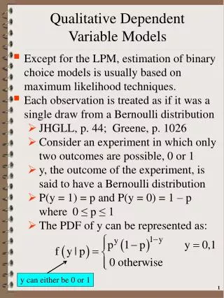
Qualitative Dependent Variable Models • Binary Choice: Yes/No decision • y=1 when choice is made y=0 when choice not made • How can we model this choice decision? • We could use our linear (CRM) model: • yt = Xtβ + et (t=1,…T) • Known as the Linear Probability Model(LPM) • Represent the LPM via the following
Qualitative Dependent Variable Models Linear Probability Model yt = Xtβ + et y E[y|X]=b0 + b1X 1 et E[y|X=xi] 0 X xi Observed Data
Qualitative Dependent Variable Models • Problems with the LPM (yt = Xtβ + et) • When y is a binary random variable, the unconditional expectation of y is the probability that the event occurs (i.e. the prob. the choice is made) • E(yt)=1*Pr(yt=1) + 0*Pr(yt=0) = Pr(yt=1) • →Under the LPM: E(yt) = E(Xtβ+et)= Xtβ = Pr(yt=1) Formula for expected value 0,1 are only values of Y Not restricted to be between 0 and 1
Qualitative Dependent Variable Models • Problems with the LPM (yt = Xtβ + et) • → constant marginal effects when depend. variable is a probability • would like to see marginal effects ↓ as the predicted prob. → 0 or 1 • The ideal probability model 1 alternative slopes at different Xtβ values 0 Xtβ • Marginal effects ↓ in absolute value sense as predicted probability approaches the probability limits
Qualitative Dependent Variable Models • Problems with the LPM • Since yt can only take two values, the error terms can only take two values for a particular value of Xt • This last characteristic implies that the error terms cannot be normally distributed given a value of X w/ Pr(Xtβ) w/ Pr(1-Xtβ)
Qualitative Dependent Variable Models • The LPM has heteroscedastic errors • Lets represent the LPM as: → E(yt) = E(1|yt = 1)Pr(yt = 1) + E(0|yt = 0)Pr(yt = 0) =1 Pr(yt=1)+0 Pr(yt=0) =Pr(yt=1) ≡ Pt = Xtβ • et=Yt-Xtβ →V(et)=E(et2)=E[(yt−Xtβ)2]=E[(yt−Pt)2] = (1− Pt)2Pr(yt= 1) + (−Pt)2Pr(yt= 0) = (1− Pt)2Pt + Pt2(1−Pt) since Pr(yt=0) = 1−Pt = (1−2Pt + Pt2)Pt + Pt2 – Pt3 = Pt – 2Pt2 + Pt3 + Pt2 – Pt3 = Pt−Pt2 = (1−Pt)Pt = (1−Xtβ) Xtβ →heteroscedastic errors as variance changes across observation →βs unbiased but inefficient
Qualitative Dependent Variable Models • Summary of Linear Probability Model • Nonsensical Predictions outside the {0,1} range • Error Terms Not Normally Distributed • Functional Form Implies Constant Marginal Effects • Error Terms are Heteroscedastic
Qualitative Dependent Variable Models • This is not directly related to our discussion of discrete choice but I thought I would mention one method that is used to guarantee predicted values coming out of an OLS model lie between 0 and 1 • Suppose you have a continuous random variable that has values between 0 and 1 (e.g., a proportion). • Lets represent this variable as P • We can use the logistic functional form to allow us to estimate a model using OLS procedures and have predicted value of P to be between 0 and 1
Qualitative Dependent Variable Models • Define the following variable • Estimate the following linear regression model: • Solving this equation for P by exponentiating both sides one obtains the following: • If β1>0, P→0 as X→−∞ and P→1 as X→∞
Qualitative Dependent Variable Models β1>0 1 Predicted value of P 0 β1Xt • Note that the marginal effect will change with the point of evaluation
Qualitative Dependent Variable Models • Instead of the LPM lets use some type of Probability Distribution to explain the variability of y Pr(yt=1) 1 Pr(y3=1) Φ(Xtβ) 0 Xt X3β X3β PDF CDF
Qualitative Dependent Variable Models • Use of a Probability Distribution • Whatever functional form used to model the probability • Model parameters like other nonlinear regression models usually are not the marginal impact of X on Pr(yt= 1) Standard normal CDF
Qualitative Dependent Variable Models • Discrete choice models are often motivated via use of an index function. • Example of decision to make a large purchase • Theoretically, the consumer makes a marginal benefit versus marginal cost calculation when deciding to purchase • Based on utilities achieved with and without making the purchase and using the funds for other purposes • Difference between benefits and costs defined as unobserved latent variable y*
Qualitative Dependent Variable Models • Latent Variable Interpretation of Discrete Choice Model • Let y* be a latent variable that is continuous with a range in value from +∞ to −∞ • Satisfies our traditional CRM assumptions about our dependent variable • Considered latent in that y* actually not observed • y* generates observed values of y’s where y is discrete (e.g., 0,1) and observed • Larger y* values generate values of y = 1 • Smaller y* values generate y = 0
Qualitative Dependent Variable Models latent variable • Latent Variable Interpretation • Lets assume that a set of exogenous variables impact y* yt*= Xtβ + et • The relationship between y, our observed discrete variable, and y* (i.e. mappingbetween y & y*) is • Lets assume that is set to 0 Pr(yt* > 0) = Pr(0+ 1Xt+et > 0) →Pr(et > −0−1Xt) = Pr(yt = 1) Assume a single X Latent Observed y*
Qualitative Dependent Variable Models yt*=Xtβ+et Pr(yt* > 0) = Pr(0+1Xt+et > 0 ) = Pr(et > -0-1Xt) = Pr(yt = 1) Pr(et > -0-1Xt)= Pr(0+1Xt+et> 0) = Pr(y*t > 0) y* E[yt*]=Xtb y=1 = 0 y=0 X x1 x2 When y* > τ, y=1 Latent error term distribution conditional on Xtβ (centered on regression line)
Qualitative Dependent Variable Models Pr(et > -0-1Xt)= Pr(y*t>0)
Qualitative Dependent Variable Models Pr(yt* > 0) = Pr(0+1Xt+et>0) = Pr(et > -0-1Xt) = Pr(yt = 1) • Use of ML techniques to obtain parameter estimates • Choose values of β0 and β1 • Such that the probability of obtaining a vector of latent errors that reflect pattern of observed 0/1 values of y is maximized • Since y* is continuous, the above avoids the problems of the LPM
Qualitative Dependent Variable Models • Since y* is unobserved, the β’s can not be estimated with CRM. • We can however use Maximum Likelihood techniques • Error terms distributed standard normal → Probit Model • Error terms distributed logistically → Logit Model • Standard Normal Random variable, Z, [Z~N(0,1)] with CDF • Logistic Random Variable, Z, with CDF
Qualitative Dependent Variable Models • With E(e|X) = 0 • Probit Model: Var(e|X)=1 • Logit Model: Var(e|X)=π2/3 • For many applications it is an arbitrary assumption as to functional form of the error term distribution 23
Qualitative Dependent Variable Models • Lets assume et distributed either logistically or normally around E(yt*|Xt) [= β0+β1Xt ] • Values of yt=1 are observed for that portion of the latent variable distribution above τ • Assume τ = 0 • For example, define the latent variable as utility difference (U*) from undertaking an activity (U1) versus not undertaking an activity(U0) • If U* = U1 - U0 > 0 → undertake the activity
Qualitative Dependent Variable Models Assume et distributed either via Logistic or Standard Normal Latent Variable: yt*=0+1Xt+et (Difference in Utility) Pr(yt* > 0) = Pr(0+1Xt+et > 0) = Pr(et > -0-1Xt) = Pr(yt = 1) Pr(et > -0-1Xt) y* E[yt*]=Xtb y=1 (et > -0-1Xt) =0 y=0 (et < -0-1Xt) et = -0-1Xt X x1 x2 yt* (latent difference in utility levels)=0
Qualitative Dependent Variable Models Pr(yt* > 0) P(yt*< 0) E[yt*] = Xtb • Even if E(yt*|Xt) is in the (pink) shaded portion where yt=1, there is still a possibility to observe a 0 if et is large and negative (yellow shaded area)
Qualitative Dependent Variable Models Assuming τ = 0 Pr(yi=1) = Pr(ei > -xi) PDF(e) Error term Distribution −Xiβ Pr(ei> −Xiβ)
Qualitative Dependent Variable Models If et distributed logistic/normal → symmetric distributions Pr(yi=1) = Pr(ei > -xi) = Pr(ei < xi) = cdf(xi) PDF(e) Symmetric Distribution [PDF(ei)] −Xiβ Xiβ Pr(ei < Xiβ) = Pr(ei> −Xiβ)
Qualitative Dependent Variable Models If et distributed logistic/normal → symmetric distribution • Pr(yi=1) = Pr(ei>-xi) = Pr(ei<xi) = cdf(xi) = Φ(xi) • The latent variable formulation produces a nonlinear probability model for Pr(y=1|X) • By construction, Pr(yi=1) lies between 0,1 because it is based on the CDF for ei 1 Pr(yi=1) xi 0 0
Qualitative Dependent Variable Models • Two comments wrt latent variable model • The assumption of a known error term variance does not impact results • The assumption of a 0 threshold does not impact model if the model contains an intercept term • Suppose the error variance is scaled by an unrestricted parameter σ2 • The latent regression is transformed to: y* = Xβ + σε and y*/σ=X(β/σ) + ε • The observed data will be unchanged where y is still 0 or 1 depending only on the sign of y* not on its scale • This means that there is no information about σ in the data so it cannot be estimated
Qualitative Dependent Variable Models • Lets look at the 0 cut-off assumption. • Let τ be an assumed non-zero threshold • Let α be the unknown constant term • Let X and β be the remaining components of the index function not including the constant term • →the probability that y (the observed data) equals 1 is: Pr(y*>τ|X) = Pr(α+Xβ+ε > τ|X) = Pr((α- τ) +Xβ+ε > 0|X) • Since α is unknown, the difference (α – τ) remains an unknown parameter and can be redefined as α* • Pr(y*>τ|X) = Pr(α*+Xβ+ε>0|X)
Qualitative Dependent Variable Models • Random Utility Application of the Latent Variable Model • Utility derived from a choice • Utility impacted by • Attributes of choice • Individual decision-maker characteristics
Qualitative Dependent Variable Models • Example of Mode Choice of Work Commute (car vs. bus) • Attributes of the Choice • Cash cost of car vs. bus • Commute time • Comfort • Safety • Attributes of the Individual • Household income • Occupation • Age structure of household vary across choice Do not vary across choice
Qualitative Dependent Variable Models • Random Utility Interpretation of Latent Variable Model • Utility derived from each choice • Ui0, Ui1 are utilities derived from the two choices (0 = bus, 1 = car) • are average (conditional) utilities • Zi0, Zi1 are characteristics of the choices perceived by ith decision-maker • i.e., commute time, comfort • Wi is a vector of socioeconomic characteristics of ith decision-maker • i.e., household income random errors
Qualitative Dependent Variable Models • Random Utility Application of the Latent Variable Model • Utilities Ui0, Ui1 are random • ith individual will make choice 1 if Ui1 – Ui0 > 0 • yi*≡ Ui1 – Ui0 • The unobservable (latent) variable, yi*is the difference in utility levels • Will make choice 1 if yi* > 0
Qualitative Dependent Variable Models • Random Utility Application of the Latent Variable Model • Remember that: same coefficient different coefficients
Qualitative Dependent Variable Models • Random Utility Application of the Latent Variable Model • Using the definition of the latent variable (yi* ≡ Ui1 – Ui0 ): y*i= (Zi1 – Zi0)δ + Wi(γ1 – γ0) + (ei1 – ei0) = Xβ + e*i • Pi = Pr(yi = 1) = Pr(y*i > 0) = Pr(e*i > – Xiβ) γ * • As before assume e*t distributed either logistically or normally around E(yt*|Xt) [= β0+β1Xt] • Values of yt=1 are observed for that portion of the latent variable distribution above τ (i.e., 0) • That is, utility difference > 0