
Understanding Newton-Cotes Integration Formulas
Learn about Newton-Cotes integration, trapezoidal and Simpson's rules, composite formulas, error estimation, MATLAB implementation, and higher-order methods.

Understanding Newton-Cotes Integration Formulas
E N D
Presentation Transcript
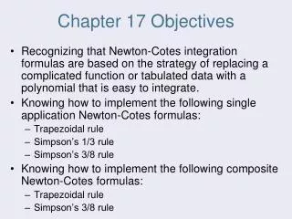
Chapter 17 Objectives • Recognizing that Newton-Cotes integration formulas are based on the strategy of replacing a complicated function or tabulated data with a polynomial that is easy to integrate. • Knowing how to implement the following single application Newton-Cotes formulas: • Trapezoidal rule • Simpson’s 1/3 rule • Simpson’s 3/8 rule • Knowing how to implement the following composite Newton-Cotes formulas: • Trapezoidal rule • Simpson’s 3/8 rule
Objectives (cont) • Recognizing that even-segment-odd-point formulas like Simpson’s 1/3 rule achieve higher than expected accuracy. • Knowing how to use the trapezoidal rule to integrate unequally spaced data. • Understanding the difference between open and closed integration formulas.
Integration • Integration:is the total value, or summation, of f(x) dx over the range from a to b:
Newton-Cotes Formulas • The Newton-Cotes formulas are the most common numerical integration schemes. • Generally, they are based on replacing a complicated function or tabulated data with a polynomial that is easy to integrate:where fn(x) is an nth order interpolating polynomial.
Newton-Cotes Examples • The integrating function can be polynomials for any order - for example, (a) straight lines or (b) parabolas. • The integral can be approximated in one step or in a series of steps to improve accuracy.
The Trapezoidal Rule • The trapezoidal rule is the first of the Newton-Cotes closed integration formulas; it uses a straight-line approximation for the function:
Error of the Trapezoidal Rule • An estimate for the local truncation error of a single application of the trapezoidal rule is:where is somewhere between a and b. • This formula indicates that the error is dependent upon the curvature of the actual function as well as the distance between the points. • Error can thus be reduced by breaking the curve into parts.
Composite Trapezoidal Rule • Assuming n+1 data points are evenly spaced, there will be n intervals over which to integrate. • The total integral can be calculated by integrating each subinterval and then adding them together:
Simpson’s Rules • One drawback of the trapezoidal rule is that the error is related to the second derivative of the function. • More complicated approximation formulas can improve the accuracy for curves - these include using (a) 2nd and (b) 3rd order polynomials. • The formulas that result from taking the integrals under these polynomials are called Simpson’s rules.
Simpson’s 1/3 Rule • Simpson’s 1/3 rule corresponds to using second-order polynomials. Using the Lagrange form for a quadratic fit of three points:Integration over the three points simplifies to:
Error of Simpson’s 1/3 Rule • An estimate for the local truncation error of a single application of Simpson’s 1/3 rule is:where again is somewhere between a and b. • This formula indicates that the error is dependent upon the fourth-derivative of the actual function as well as the distance between the points. • Note that the error is dependent on the fifth power of the step size (rather than the third for the trapezoidal rule). • Error can thus be reduced by breaking the curve into parts.
Composite Simpson’s 1/3 Rule • Simpson’s 1/3 rule can be used on a set of subintervals in much the same way the trapezoidal rule was, except there must be an odd number of points. • Because of the heavy weighting of the internal points, the formula is a little more complicated than for the trapezoidal rule:
Simpson’s 3/8 Rule • Simpson’s 3/8 rule corresponds to using third-order polynomials to fit four points. Integration over the four points simplifies to: • Simpson’s 3/8 rule is generally used in concert with Simpson’s 1/3 rule when the number of segments is odd.
Higher-Order Formulas • Higher-order Newton-Cotes formulas may also be used - in general, the higher the order of the polynomial used, the higher the derivative of the function in the error estimate and the higher the power of the step size. • As in Simpson’s 1/3 and 3/8 rule, the even-segment-odd-point formulas have truncation errors that are the same order as formulas adding one more point. For this reason, the even-segment-odd-point formulas are usually the methods of preference.
Integration with Unequal Segments • Previous formulas were simplified based on equispaced data points - though this is not always the case. • The trapezoidal rule may be used with data containing unequal segments:
MATLAB Functions • MATLAB has built-in functions to evaluate integrals based on the trapezoidal rule • z = trapz(y)z = trapz(x, y)produces the integral of y with respect to x. If x is omitted, the program assumes h=1. • z = cumtrapz(y)z = cumtrapz(x, y)produces the cumulative integral of y with respect to x. If x is omitted, the program assumes h=1.
Multiple Integrals • Multiple integrals can be determined numerically by first integrating in one dimension, then a second, and so on for all dimensions of the problem.
Chapter 18 Objectives • Understanding how Richardson extrapolation provides a means to create a more accurate integral estimate by combining two less accurate estimates. • Understanding how Gauss quadrature provides superior integral estimates by picking optimal abscissas at which to evaluate the function. • Knowing how to use MATLAB’s built-in functions quad and quadl to integrate functions.
Richardson Extrapolation • Richard extrapolation methods use two estimates of an integral to compute a third, more accurate approximation. • If two O(h2) estimates I(h1) and I(h2) are calculated for an integral using step sizes of h1 and h2, respectively, an improved O(h4) estimate may be formed using: • For the special case where the interval is halved (h2=h1/2), this becomes:
Richardson Extrapolation (cont) • For the cases where there are two O(h4) estimates and the interval is halved (hm=hl/2), an improved O(h6) estimate may be formed using: • For the cases where there are two O(h6) estimates and the interval is halved (hm=hl/2), an improved O(h8) estimate may be formed using:
The Romberg Integration Algorithm • Note that the weighting factors for the Richardson extrapolation add up to 1 and that as accuracy increases, the approximation using the smaller step size is given greater weight. • In general,where ij+1,k-1 and ij,k-1 are the more and less accurate integrals, respectively, and ij,k is the new approximation. k is the level of integration and j is used to determine which approximation is more accurate.
Romberg Algorithm Iterations • The chart below shows the process by which lower level integrations are combined to produce more accurate estimates:
Gauss Quadrature • Gauss quadrature describes a class of techniques for evaluating the area under a straight line by joining any two points on a curve rather than simply choosing the endpoints. • The key is to choose the line that balances the positive and negative errors.
Gauss-Legendre Formulas • The Gauss-Legendre formulas seem to optimize estimates to integrals for functions over intervals from -1 to 1. • Integrals over other intervals require a change in variables to set the limits from -1 to 1. • The integral estimates are of the form:where the ci and xi are calculated to ensure that the method exactly integrates up to (2n-1)th order polynomials over the interval from -1 to 1.
Adaptive Quadrature • Methods such as Simpson’s 1/3 rule has a disadvantage in that it uses equally spaced points - if a function has regions of abrupt changes, small steps must be used over the entire domain to achieve a certain accuracy. • Adaptive quadrature methods for integrating functions automatically adjust the step size so that small steps are taken in regions of sharp variations and larger steps are taken where the function changes gradually.
Adaptive Quadrature in MATLAB • MATLAB has two built-in functions for implementing adaptive quadrature: • quad: uses adaptive Simpson quadrature; possibly more efficient for low accuracies or nonsmooth functions • quadl: uses Lobatto quadrature; possibly more efficient for high accuracies and smooth functions • q = quad(fun, a, b, tol, trace, p1, p2, …) • fun : function to be integrates • a, b: integration bounds • tol: desired absolute tolerance (default: 10-6) • trace: flag to display details or not • p1, p2, …: extra parameters for fun • quadl has the same arguments
Chapter 19 Objectives • Understanding the application of high-accuracy numerical differentiation formulas for equispaced data. • Knowing how to evaluate derivatives for unequally spaced data. • Understanding how Richardson extrapolation is applied for numerical differentiation. • Recognizing the sensitivity of numerical differentiation to data error. • Knowing how to evaluate derivatives in MATLAB with the diff and gradient functions. • Knowing how to generate contour plots and vector fields with MATLAB.
Differentiation • The mathematical definition of a derivative begins with a difference approximation:and as x is allowed to approach zero, the difference becomes a derivative:
High-Accuracy Differentiation Formulas • Taylor series expansion can be used to generate high-accuracy formulas for derivatives by using linear algebra to combine the expansion around several points. • Three categories for the formula include forward finite-difference, backward finite-difference, and centered finite-difference.
Richardson Extrapolation • As with integration, the Richardson extrapolation can be used to combine two lower-accuracy estimates of the derivative to produce a higher-accuracy estimate. • For the cases where there are two O(h2) estimates and the interval is halved (h2=h1/2), an improved O(h4) estimate may be formed using: • For the cases where there are two O(h4) estimates and the interval is halved (h2=h1/2), an improved O(h6) estimate may be formed using: • For the cases where there are two O(h6) estimates and the interval is halved (h2=h1/2), an improved O(h8) estimate may be formed using:
Unequally Spaced Data • One way to calculated derivatives of unequally spaced data is to determine a polynomial fit and take its derivative at a point. • As an example, using a second-order Lagrange polynomial to fit three points and taking its derivative yields:
Derivatives and Integrals for Data with Errors • A shortcoming of numerical differentiation is that it tends to amplify errors in data, whereas integration tends to smooth data errors. • One approach for taking derivatives of data with errors is to fit a smooth, differentiable function to the data and take the derivative of the function.
Numerical Differentiation with MATLAB • MATLAB has two built-in functions to help take derivatives, diff and gradient: • diff(x) • Returns the difference between adjacent elements in x • diff(y)./diff(x) • Returns the difference between adjacent values in y divided by the corresponding difference in adjacent values of x
Numerical Differentiation with MATLAB • fx = gradient(f, h)Determines the derivative of the data in f at each of the points. The program uses forward difference for the first point, backward difference for the last point, and centered difference for the interior points. h is the spacing between points; if omitted h=1. • The major advantage of gradient over diff is gradient’s result is the same size as the original data. • Gradient can also be used to find partial derivatives for matrices: [fx, fy] = gradient(f, h)
Visualization • MATLAB can generate contour plots of functions as well as vector fields. Assuming x and y represent a meshgrid of x and y values and z represents a function of x and y, • contour(x, y, z) can be used to generate a contour plot • [fx, fy]=gradient(z,h) can be used to generate partial derivatives and • quiver(x, y, fx, fy) can be used to generate vector fields
Chapter 20 Objectives • Understanding the meaning of local and global truncation errors and their relationship to step size for one-step methods for solving ODEs. • Knowing how to implement the following Runge-Kutta (RK) methods for a single ODE: • Euler • Heun • Midpoint • Fourth-Order RK • Knowing how to iterate the corrector of Heun’s method. • Knowing how to implement the following Runge-Kutta methods for systems of ODEs: • Euler • Fourth-order RK
Ordinary Differential Equations • Methods described here are for solving differential equations of the form: • The methods in this chapter are all one-step methods and have the general format:where is called an increment function, and is used to extrapolate from an old value yi to a new value yi+1.
Euler’s Method • The first derivative provides a direct estimate of the slope at ti:and the Euler method uses that estimate as the increment function:
Error Analysis for Euler’s Method • The numerical solution of ODEs involves two types of error: • Truncation errors, caused by the nature of the techniques employed • Roundoff errors, caused by the limited numbers of significant digits that can be retained • The total, or global truncation error can be further split into: • local truncation error that results from an application method in question over a single step, and • propagated truncation error that results from the approximations produced during previous steps.
Error Analysis for Euler’s Method • The local truncation error for Euler’s method is O(h2) and proportional to the derivative of f(t,y) while the global truncation error is O(h). • This means: • The global error can be reduced by decreasing the step size, and • Euler’s method will provide error-free predictions if the underlying function is linear. • Euler’s method is conditionally stable, depending on the size of h.
Heun’s Method • One method to improve Euler’s method is to determine derivatives at the beginning and predicted ending of the interval and average them: • This process relies on making a prediction of the new value of y, then correcting it based on the slope calculated at that new value. • This predictor-corrector approach can be iterated to convergence:
Midpoint Method • Another improvement to Euler’s method is similar to Heun’s method, but predicts the slope at the midpoint of an interval rather than at the end: • This method has a local truncation error of O(h3) and global error of O(h2)
Runge-Kutta Methods • Runge-Kutta (RK) methods achieve the accuracy of a Taylor series approach without requiring the calculation of higher derivatives. • For RK methods, the increment function can be generally written as:where the a’s are constants and the k’s arewhere the p’s and q’s are constants.


![WATER GARDENS, PLANTS, AND ALGAE – Chapter 17 [objectives]](https://cdn2.slideserve.com/5323854/water-gardens-plants-and-algae-chapter-17-objectives-dt.jpg)