Download
1 / 23
320 likes | 788 Views
The Leslie Matrix How do we take the differences in survivorship and fecundity into account to ‘project’ the future of the population?

E N D
The Leslie Matrix How do we take the differences in survivorship and fecundity into account to ‘project’ the future of the population? The mechanism is to re-cast the life table into a matrix form – called the Leslie matrix. The product of that matrix multiplying a column vector that presents the age structure of the population projects the population Nt into the structure of the population Nt+1. That is too dense to fully understand. Here’s how the matrix and multiplication develop…
The first thing to note is that if we want to know how many individuals are x+1 years old next year, we need to know how many x year olds there are this year and what fraction of them survive. We already know survivorships lx and lx+1. They are the fractions of the original cohort alive at each age. To calculate the fraction of age class x alive at age x+1, we use a new variable, px: px = lx+1/lx Let’s now add px to the life table from before, and also show how you can use the p’s and age class sizes to project the population forward:
Age x#alivelxmx px FxNt+1 0 100 1.000 0 .8 0 ntpxmx 1 80 .800 .2 .75 .15 n0p0 2 60 .600 .3 .66 .198 n1p1 3 40 .400 1.0 1.0 1.0 n2p2 4 40 .400 .6 .5 .3 n3p3 5 20 .200 .1 --- --- n4p4 6 0 --- --- --- --- --- What is new here is the calculation of the number of newborns. We first calculate a fertility for each age class, Fi, which is, for age class i, the product of the mi and pi. This product is the number of offspring produced by a female which survived to reach the age/period discounted by the probability of survival through the period.
Once you have the 'discounted' fertilities for each age class, the total number of newborns in the next period is the sum of products of fertilities times population numbers for all age classes: n0,t+1 = Fxnx,t We can now organize the ‘new’ life table information into a Leslie matrix. The matrix has the fertilities (Fx) for age classes as its first row and the proportional survivorships (px) as subdiagonal elements. Here’s what the matrix looks like, using the abstraction of Fxs and pxs:
In general terms: F0 F1 F2 F3 F4 F5 p0 0 0 0 0 0 0 p1 0 0 0 0 0 0 p2 0 0 0 0 0 0 p3 0 0 0 0 0 0 p4 0 For our specific matrix: 0 .15 .198 1 .3 0 .8 0 0 0 0 0 0 .75 0 0 0 0 0 0 .66 0 0 0 0 0 0 1 0 0 0 0 0 0 .5 0
Now if we post-multiply this matrix by a matrix (really a column vector) which is the age-class structure at time t, we'll get a new column vector which is the age structure at time t+1. To see that, here is the general pattern and rules for multiplying matrices: The product only exists if the number of columns in the first matrix equals the number of rows in the second. The process is also intransitive, i.e. A x B is not equal to B x A. Each element in the product matrix (C) which results from multiplication is the sum of the products of corresponding elements in the row of matrix A and the column of matrix B. In standard notation:
In abstract terms: To illustrate, the product of two 2x2 matrices is shown below, with the individual row by column products displayed in the result. |1 2| x |5 6| = |5+14 6+16 | = |19 22| |3 4| |7 8| |15+28 18+32| |43 50| To demonstrate intransitivity, here’s the multiplication with the matrices reversed: |5 6| x |1 2| = |5+18 10+24| = |23 34| |7 8| |3 4| |7+24 14+32| |31 46|
Now let’s briefly review the population projection value of the Leslie matrix: L x Nt = Nt+1 and Nt+2 = L x Nt+1 = L x (L x Nt) = L2Nt Since L doesn’t change with density, … In many plants it is not age that determines their survivorship and reproduction, but the stage they have reached. Now instead of ages setting the rows of a projection matrix, it is the sequence of stages. The first row of the matrix is the fecundities of the stages. Instead of the survivorships, what goes below the first row is what are called transition probabilities. The matrix is called a Lefkovitch matrix.
Nt+1 = ANt • A is a Lefkovitch or transition matrix • It contains all stage- specific rates of transition and seed production • There are i columns and j (= i) rows for a population with i stages If i = j the value indicates the fraction of organisms that remain in the same stage.
We could use the teasel data to produce a Lefkovitch matrix, but we’ll use a much simpler case of Coryphanthum robbinsorum, an endangered cactus from the Sonoran desert. This cactus has no seed bank, so that annual census would not detect seeds, and we can use a fecundity measure that incorporates not just seeds produced, but probability of seeds germinating and surviving to the time of the census.
The result is this simplified life cycle graph, which is the equivalent of the diagrammatic life tables you saw earlier… Since this model doesn’t include a seed stage, consider how we determine the number of small juveniles at the ‘next’ census: n1(t+1) = p11n1 + n3(t)F
Here’s the basic matrix projection equation: n1(t+1) p11 0 F n1(t) n2(t+1) = p21 p22 0 x n2(t) n3(t+1) 0 p32 p33 n3(t) Here are the values for the Lefkovitch matrix for one of the three sites collected by Schmalzel (1995): p11 0 F 0.434 0 0.560 p21 p22 0 = 0.333 0.610 0 0 p32 p33 0 0.304 0.956 From this matrix you can calculate various important things about the population: the stable age distribution – in the figure below this matrix describes the population at site C, the only one where a fairly large proportion of small juveniles grow to large juveniles and mature to reproduce.
That difference in the proportion growing and maturing also produces a larger for site C (1.12, indicating a growing population, versus 0.998 and 0.997, indicating declining populations at the other sites). is the dominant (largest) eigenvalue of the matrix. There are additional, smaller eigenvalues as solutions to the polynomial equation that is used to determine the eigenvalues (the roots of the polynomial equation).
Even before the population has reached a SAD and a stable growth rate, the growth can be predicted from eigenvalues and eigenvectors (Caswell, 2001) according to the formula: where the c values are constants set by initial population structure. For site C the eigenvalues and eigenvectors can be plotted over time. The plots show that the observed population growth is explained by the dominant eigenvalue (component 1) after only a very few years. The other components (eigenvalues) converge on 0 contribution…
The left eigenvector of the Lefkovitch (or Leslie) matrix gives proportions in each ‘age class’ in a SAD when age classes are appropriate, or here the stable relative stage abundances, and the right eigenvector gives reproductive values.
The reproductive values for site C Coryphantha robbinsorum are: small juveniles 1 large juveniles 2.06 adults 3.44 How sensitive are these results to small changes in survivorship or transition probabilities? The matrices can also be used to determine that. Each element aij of A (or the Leslie matrix, i.e. the p’s or fecundities) has an associated sensitivity value sij. s indicates populations most vulnerable points that may be manipulated in order to manipulate . Because may be used to estimate phenotypic fitness, sij indicates how changes in aij will affect fitness.
A high sij suggests that natural selection should act on characters affecting that aijbecause small differences between genotypes will affect their fitness. The sensitivity value sij for matrix element aij is: sij = vicj/v,c v,c is the scalar product of the right and left eigenvectors. It is a constant value across all elements in the vectors. aij values themselves can vary in size, over the range 0 1 for proportional survivorships, but over a wide range for fecundities. Sensitivity is assessed for a fixed small change in aij. That makes comparison of sij values for fecundities and survivorships difficult.
To deal with that problem, there is a better measure, called elasticity. This measure is scaled to indicate the relative impact of each aij to . Elasticities for a Lefkovitch (or a Leslie) matrix sum to 1. They therefore measure the relative contributions of each element of the matrix to the growth rate (), tested by unit change in each, all other elements held constant. As is evident in the figure, it is survivorship as adults that largely determines growth rate in this cactus at all sites…
There remains the example of teasel, Dipsacus fullonum ... First, here are the stages into which the teasel life history is subdivided: n1 - dormant seeds in year 1 n2 - dormant seeds in year 2 n3 - small rosettes n4 - medium rosettes n5 - large rosettes n6 - flowering plants The matrix which results differs slightly among individual fields studied. The values, particularly reflecting what was found in field A of the study, were:
0 0 0 0 0 322.38 • 0.966 0 0 0 0 0 • 0.013 0.010 0.125 0 0 3.448 • 0.007 0 0.125 0.238 0 30.170 • 0.008 0 0.036 0.245 0.167 0.862 • 0 0 0 0.023 0.750 0 • There are lot’s more numbers here. What do they all mean? • 0.966 of the seeds which were dormant in the first • year remain dormant until at least the beginning of • the second year. • b) 0.013 of the seeds which were dormant through the winter germinate and become small rosettes in the first year.
c) 0.007 of the seeds which were dormant through their first winter grow in the next year to become medium rosettes, and the next number, 0.008, represents the fraction which grew to become large rosettes in their first growth season. d) Now look at the 3rd column. The two 0.125s represent the fraction which remain in the small rosette category (upper one) and the fraction which advance to become medium rosettes. The 0.036 represents the fraction which grow so rapidly that they become large rosettes in their first year of growth.
e) Similarly, the 4th column includes values for remaining in the medium rosette category, growing to become large rosettes, and the small fraction which reach the large category so early in the season that they proceed to flower. f) The last column may be initially confusing. If we wrote the matrix without correction, there would be only one non-zero value in it: the average number of seeds produced by a flowering plant, since Dipsacus is a biennial which dies after flowering. That number would have been 431 seeds per plant. However, correction recognizes that some seeds are not dormant in their first year.
The fraction which enter dormancy is 0.749. Thus the proper value for seeds produced to enter the first category, seeds dormant in their first year, is 431 x 0.749 = 322.38. The other numbers reflect seeds which germinate and begin growth in their first year, rather than becoming dormant. The fraction germinating and becoming small rosettes is 0.008, which, multiplied by the total seed production (431), gives 3.448. The number which grow to medium rosettes is 30.170, and the number which grow all the way to large rosettes is 0.862. As you might expect of biennials, none flower in their first year.