Functional Genomics and Microarray Analysis (2)
Functional Genomics and Microarray Analysis (2). Data Clustering Lecture Overview. Introduction: What is Data Clustering Key Terms & Concepts Dimensionality Centroids & Distance Distance & Similarity measures Data Structures Used Hierarchical & non-hierarchical Hierarchical Clustering

Functional Genomics and Microarray Analysis (2)
E N D
Presentation Transcript
Data ClusteringLecture Overview • Introduction: What is Data Clustering • Key Terms & Concepts • Dimensionality • Centroids & Distance • Distance & Similarity measures • Data Structures Used • Hierarchical & non-hierarchical • Hierarchical Clustering • Algorithm • Single/complete/average linkage • Dendrograms • K-means Clustering • Algorithm • Other Related Concepts • Self Organising Maps (SOM) • Dimensionality Reduction: PCA & MDS
Gene Expression Matrix Samples Genes Gene expression levels IntroductionAnalysis of Gene Expression Matrices • In a gene expression matrix, rows represent genes and columns represent measurements from different experimental conditions measured on individual arrays. • The values at each position in the matrix characterise the expression level (absolute or relative) of a particular gene under a particular experimental condition.
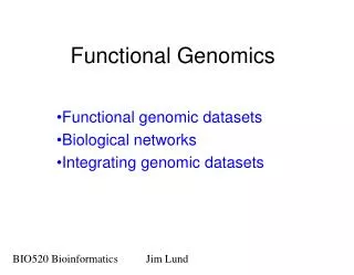
IntroductionIdentifying Similar Patterns • The goal of microarray data analysis is to find relationships and patterns in the data to achieve insights in underlying biology. • Clustering algorithms can be applied to the resulting data to find groups of similar genes or groups of similar samples. • e.g. Groups of genes with “similar expression profiles (Co-expressed Genes) --- similar rows in the gene expression matrix • or Groups of samples (disease cell lines/tissues/toxicants) with “similar effects” on gene expression --- similar columns in the gene expression matrix
IntroductionWhat is Data Clustering • Clustering of data is a method by which large sets of data is grouped into clusters (groups) of smaller sets of similar data. • Example: There are a total of 10 balls which are of three different colours. We are interested in clustering the balls into three different groups. • An intuitive solution is that balls of same colour are clustered (grouped together) by colour • Identifying similarity by colour was easy, however we want to extend this to numerical values to be able to deal with gene expression matrices, and also to cases when there are more features (not just colour).
IntroductionClustering Algorithms • A clustering algorithm attempts to find natural groups of components (or data) based on some notion similarity over the features describing them. • Also, the clustering algorithm finds the centroid of a group of data sets. • To determine cluster membership, many algorithms evaluate the distance between a point and the cluster centroids. • The output from a clustering algorithm is basically a statistical description of the cluster centroids with the number of components in each cluster.
Gene Expression Matrix Samples Genes Gene expression levels Key Terms and ConceptsDimensionality of gene expression matrix • Clustering algorithms work by calculating distances (or alternatively similarity in higher-dimensional spaces), i.e. when the elements are described by many features (e.g. colour, size, smoothness, etc for the balls example) • A gene expression matrix of N Genes x M Samples can be viewed as: • N genes, each represented in an M-dimensional space. • M samples, each represented in N-dimensional space • We will show graphical examples mainly in 2-D spaces • i.e. when N= 2 or M=2
centroid gene A + + + + + + + + + + + + + + + + + + + + + + + + + gene B Key Terms and ConceptsCentroid and Distance • In the first example (2 genes & 25 samples) the expression values of 2 Genes are plotted for 25 samples and Centroid shown) • In the second (2 genes & 2 samples) example the distance between the expression values of the 2 genes is shown
Key Terms and ConceptsCentriod and Distance Cluster centroid : The centroid of a cluster is a point whose parameter values are the mean of the parameter values of all the points in the clusters. Distance: Generally, the distance between two points is taken as a common metric to assess the similarity among the components of a population. The commonly used distance measure is the Euclidean metric which defines the distance between two points p= ( p1, p2, ....) and q = ( q1, q2, ....) is given by :
(x2,y2) (x1, y1) Key Terms and ConceptsDistance/Similarity Measures • Euclidean (L2) distance • Manhattan (L1) distance • Lm: (|x1-x2|m+|y1-y2|m)1/m • L∞: max(|x1-x2|,|y1-y2|) • Inner product: x1x2+y1y2 • Correlation coefficient • Spearman rank correlation coefficient • For simplicity we will concentrate on Euclidean and Manhattan distances in this course
Key Terms and ConceptsDistance/Similarity Matrices • Gene Expression Matrix • N Genes x M Samples • Clustering is based on distances, this leads to a new useful data structure: • Similarity/Dissimilarity matrix • Represents the distance between either N Genes (NxN) or M Samples (MxM) • Only need half the matrix, since it is symmetrical
Key TermsHierarchical vs. Non-hierarchical • Hierarchical clustering is the most commonly used methods for identifying groups of closely related genes or tissues. Hierarchical clustering is a method that successively links genes or samples with similar profiles to form a tree structure – much like phylognentic tree. • K-means clustering is a method for non-hierarchical (flat) clustering that requires the analyst to supply the number of clusters in advance and then allocates genes and samples to clusters appropriately.
Hierarchical ClusteringAlgorithm • Given a set of N items to be clustered, and an NxN distance (or similarity) matrix, the basic process hierarchical clustering is this: • Start by assigning each item to its own cluster, so that if you have N items, you now have N clusters, each containing just one item. • Find the closest (most similar) pair of clusters and merge them into a single cluster, so that now you have one less cluster. • Compute distances (similarities) between the new cluster and each of the old clusters. • Repeat steps 2 and 3 until all items are clustered into a single cluster of size N.
1 2 3 Hierarchical Cluster Analysis • Scan matrix for minimum • Join genes to 1 node • Update matrix
Average distance Min distance Max distance Hierarchical ClusteringDistance Between Two Clusters • Single-Link Method / Nearest Neighbor • Complete-Link / Furthest Neighbor • Their Centroids. • Average of all cross-cluster pairs. Whereas it is straightforward to calculate distance between two points, we do have various options when calculating distance between clusters.
Key TermsLinkage Methods for hierarchical clustering • Single-link clustering (also called the connectedness or minimum method) : we consider the distance between one cluster and another cluster to be equal to the shortest distance from any member of one cluster to any member of the other cluster. If the data consist of similarities, we consider the similarity between one cluster and another cluster to be equal to the greatest similarity from any member of one cluster to any member of the other cluster. • Complete-link clustering (also called the diameter or maximum method): we consider the distance between one cluster and another cluster to be equal to the longest distance from any member of one cluster to any member of the other cluster. • Average-link clustering we consider the distance between one cluster and another cluster to be equal to the average distance from any member of one cluster to any member of the other cluster.
Single-Link Method Euclidean Distance a a,b b a,b,c a,b,c,d c d c d d (1) (3) (2) Distance Matrix
Complete-Link Method Euclidean Distance a a,b a,b b a,b,c,d c,d c d c d (1) (3) (2) Distance Matrix
0 2 4 6 Single-Link Complete-Link Key Terms and ConceptsDendrograms and Linkage The resulting tree structure is usally referred to as a dendrogram. In a dendrogram the length of each tree branch represents the distance between clusters it joins. Different dendrograms may arise when different Linkage methods are used
Two Way Hierarchical Clustering Note we can do two way clustering by performing clustering on both the rows and the columns It is common to visualise the data as shown using a heatmap. Don’t confuse the heatmap with the colours of a microarray image. They are different ! Why?
K-Means Clustering • Basic Ideas : using cluster centroids (means) to represent cluster • Assigning data elements to the closet cluster (centroid). • Goal: Minimise square error (intra-class dissimilarity)
1) Select an initial partition of k clusters 2) Assign each object to the cluster with the closest centroid 3) Compute the new centeroid of the clusters: 4) Repeat step 2 and 3 until no object changes cluster K-means ClusteringAlgorithm
Summary • Clustering algorithms used to find similarity relationships between genes, diseases, tissue or samples • Different similarity metrics can be used – mainly Euclidean and Manhattan) • Hierarchical clustering • Similarity matrix • Algorithm • Linkage methods • K-means clustering algorithm
Data ClassificationLecture Overview • Introduction: Diagnostic and Prognostic Tools • Data Classification • Classification vs. Classification • Examples of Simple Classification Algorithms • Centroid-based • K-NN • Decision Trees • Basic Concept • Algorithm • Entropy and Information Gain • Extracting rules from trees • Bayesian Classifiers • Evaluating Classifiers
IntroductionPredictive Modelling • Diagnostic Tools: One of the most exciting areas of Microarray research is the use of Microarrays to find groups of gene that can be used diagnostically to determine the disease that an individual is suffering. • Tissue Classification Tools: a simple example is given measurements from one tissue type is to be able to ascertain whether the tissue has markers of cancer or not, and if so which type of cancer. • Prognostic Tools: Another exciting area is given measurements from an individual’s sample is to prognostically predict the success of a course of a particular therapy • In both cases we can train a classification algorithm on previously collected data so as to obtain a predictive modelling tool. The aim of the algorithm is to find a small set of features and their values (e.g. set of genes and their expression values) that can be used in future predictions (or classification) on unseen samples
Classification:Obtaining a labeled training data set • Goal: Identify subset of genes that distinguish between treatments, tissues, etc. • Method • Collect several samples grouped by type (e.g. Diseased vs. Healthy) or by treatment outcome (e.g. Success vs. Failure). • Use genes as “features” • Build a classifier to distinguish treatments ID G1 G2 G3 G4 Cancer 1 11.12 1.34 1.97 11.0 No 2 12.34 2.01 1.22 11.1 No 3 13.11 1.34 1.34 2.0 Yes 4 13.34 11.11 1.38 2.23 Yes 5 14.11 13.10 1.06 2.44 Yes 6 11.34 14.21 1.07 1.23 No 7 21.01 12.32 1.97 1.34 Yes 8 66.11 33.3 1.97 1.34 Yes 9 33.11 44.1 1.96 11.23 Yes To Predict categorical class labels construct a model based on the training set, and then use the model in classifying new unseen data
G1 <=22 >22 G3 G4 <=52 <=12 >12 >52 Yes No Yes No Classification:Generating a predictive model • The output of a classifier is a predictive model that can be used to classify unseen based on the values of their gene expressions. • The model shown below is a special type of classification models, known a Decision Tree.
Task: determine which of a fixed set of classes an example belongs to Inductive Learning System: Input: training set of examples annotated with class values. Output:induced hypotheses (model/concept description/classifiers) ClassificationOverview Learning : Induce classifiers from training data Inductive Learning System Training Data: Classifiers (Derived Hypotheses)
ClassificationOverview • Using a Classifier for Prediction Using Hypothesis for Prediction: classifying any example described in the same manner as the data used in training the system (i.e. same set of features) Classifier Decision on class assignment Data to be classified
Outlook Sunny Overcast Rain Humidity Wind Yes true Normal High false No Yes No Yes ClassificationExamples in all walks of life The values of the features in the table can be categorical or numerical. However, we only deal with categorical variables in this course The Class Value has to be Categorical.
Clustering Classification • unknown number of classes • known number of classes • based on a training set • no prior knowledge • used to classify future observations • used to understand (explore) data • Classification is a form of supervised learning • Clustering a form of unsupervised learning Classification vs. Clustering
Typical Classification Algorithms • Centroid Classifiers • kNN: k Nearest Neigbours • Bayesian Classification: Naïve Bayes and Bayesian Networks • Decision trees • Neural Networks • Linear Discriminant Analysis • Support Vector Machines • …..
Linear Classifier: Non Linear Classifier: G1 * * o o * o * o o * G1 o * * * * o o * * o * * o o o * o * o o * o * * a*G1 + b*G2 > t -> o ! * * o o * o * o G2 A linear discriminant in 2-D is a straight line. In N-D it is a hyperplace Types of ClassifiersLinear vs. non linear G2 • Linear Classifiers are easier to develop e.g Linear Discriminant Analysis (LDA) Method, which tries to find a good regression line by minimising the squared errors of the training data • Linear Classifiers, however, may produce models that are not perfect on the training data. • Non-linear classifiers tend to be more accurate, may over-fit the data • By over-fitting the data, they may actually perform worse on unseen data
_ _ + _ _ _ . + _ + + + _ + x + _ _ _ + _ + + Types of ClassifiersK-Nearest Neighbour Classifiers • K-NN works by assigning a data point to the class of its k closest neighbors (e.g. based on Euclidean or Manhattan distance). • K-NN returns the most common class label among the k training examples nearest tox. • We usually set K > 1 to avoid outliers • Variations: • Can also use a radius threshold rather than K. • We can also set a weight for each neighbour that takes into account how far it is from the query point • Model Training: None. • Classification: • Given a data point, Locate K nearest points. • Assign the majority class of the K points
Outlook Sunny Overcast Rain Humidity Wind Yes true Normal High false No Yes No Yes Types of ClassifiersDecision Trees • Decision tree • A flow-chart-like tree structure • Internal node denotes a test on an attribute • Branch represents an outcome of the test • Leaf nodes represent class labels or class distribution • Decision tree generation • At start, all the training examples are at the root • Partition examples recursively based on selected attributes • Use of decision tree: Classifying an unknown sample • Test the attribute values of the sample against the decision tree
Outlook Sunny Overcast Rain Humidity Wind Yes true Normal High false No Yes No Yes Types of ClassifiersDecision Tree Construction • General idea: • Using the training data, choose the best feature to be used for the logical test at the root of the tree. • Partition training data into sub-groups based on the values of the logical test • Recursively apply the same procedure (select attribute and split) and terminate when all the data elements in one branch are of the same class. • Key to Success is how to choose the best feature at each step • The basic approach to select a attribute is to examine each attribute and evaluate its likelihood for improving the overall decision performance of the tree. • The most widely used node-splitting evaluation functions work by reducing the degree of randomness or ‘impurity” in the current node.
Decision Tree ConstructionAlgorithm • Basic algorithm (a greedy algorithm) • Tree is constructed in a top-down recursive manner • At start, all the training examples are at the root • Attributes are categorical (if continuous-valued, they are discretized in advance) • Examples are partitioned recursively based on selected attributes • Test attributes are selected on the basis of a heuristic or statistical measure (e.g., information gain) • Conditions for stopping partitioning • All samples for a given node belong to the same class • There are no remaining attributes for further partitioning – majority voting is employed for classifying the leaf • There are no samples left
Decision TreeExample In the simple example shown, the expression values which are usually numbers have been made into discrete values. There are more complex methods that can deal with numeric features, but are beyond this course In the example, I have chosen to use 3 discrete ranges for Gene1, two ranges (high/low) for genes 2 and , and expressed (yes/no) for gene 3.
Decision TreesUsing Information Gain • Select the attribute with the highest information gain • Assume there are two classes, P and N • Let the set of examples S contain p elements of class P and n elements of class N • The amount of information (entropy) :
Information Gain in Decision Tree Construction • Assume that using attribute A a set S will be partitioned into sets {S1, S2 , …, Sv} • If Si contains piexamples of P and ni examples of N, the expected information (total entropy) in all subtrees Si generated by the partition via A is • The encoding information that would be gained by branching on A
Class P: diseased = “yes” Class N: diseased = “no” I(p, n) = I(9, 5) =0.940 Compute the entropy for G1: Hence Similarly Attribute Selection by Information Gain Computation
Extracting Classification Rules from Trees • Decision Trees can be simplified by representing the knowledge in the form of IF-THEN rules that are easier for humans to understand • One rule is created for each path from the root to a leaf • Each attribute-value pair along a path forms a conjunction • The leaf node holds the class prediction • Example IF G1 = “<=30” AND G3 = “no” THEN diseased = “no” IF G1 = “<=30” AND G3 = “yes” THEN diseased = “yes” IF G1 = “31…40” THEN diseased = “yes” IF G1 = “>40” AND G4 = “high” THEN diseased = “yes” IF G1 = “>40” AND G4 = “low” THEN diseased = “no”
Further Notes • We have mainly used examples with two classes in our examples, however most classification algorithms can work on many class values so long as they are discrete. • We have also mainly concentrated on examples that work on discrete feature values • Note that in many cases, the data may be of very high dimensionality, and this may cause problems for the algorithms, and might need to use dimensionality reduction methods.
Summary • Classification algorithms can be used to develop diagnostic and prognostic tools based on collected data by generating predictive models that can label unseen data into existing classes. • Simple classification methods: LDA, Centroid-based classifiers and k-NN • Decision Trees: • Decision Tree Induction works by choosing the best logical test for each tree node one at a time, and recursively splitting the data and applying same procedure • Entropy and Information Gain are the key concepts to apply • Not all classifiers generate 100% accuracy, confusion matrices can be used to evaluate their accuracy.