Download

1 / 50
520 likes | 717 Views
The Long-term Variation of Solar Activity. Leif Svalgaard HEPL, Stanford University STEL, Nagoya, 16 January, 2012. Indicators of Solar Activity. Sunspot Number (and Area, Magnetic Flux) Solar Radiation (TSI, UV, …, F10.7) Cosmic Ray Modulation Solar Wind Geomagnetic Variations Aurorae

E N D
The Long-term Variation of Solar Activity Leif Svalgaard HEPL, Stanford University STEL, Nagoya, 16 January, 2012
Indicators of Solar Activity • Sunspot Number (and Area, Magnetic Flux) • Solar Radiation (TSI, UV, …, F10.7) • Cosmic Ray Modulation • Solar Wind • Geomagnetic Variations • Aurorae • Ionospheric Parameters • Climate? • More… Longest direct observations Rudolf Wolf After Eddy, 1976
Use of Sunspot Number in Climate Research The Sunspot Number is used as basic input to reconstructions of Total Solar Irradiance (TSI). This fact is often ‘hidden’ by saying that the solar magnetic flux has been ‘modeled’ and that the model and reconstruction are ‘physics-based’. ‘Traditional’ View 1700 1600 1700 1800 2000 1900 1800 1900 2000 1600 Effect on Temperature J. Harder Krivova, 2010 Calahan, 2011 Many reconstructions exhibit a significant, gradual secular increase in solar activity. I shall show that this picture is probably not correct.
The Modern Grand Maximum ? Derived from Group Sunspot Number S&C Geomagnetic 4
The Modern Grand Maximum ? Derived from Group Sunspot Number S&C Geomagnetic 5
‘Modern Grand Maximum’ sometimes portrayed as Extreme Highest in 8000, or 10,000 or 12,000 years 10 Be last 2000 years 10 Be and 14 C similar last 2000 years
The Tale of Two Sunspot Numbers WSN = 10 * Groups + Spots GSN = 12 * Groups Group SSN Wolf SSN The ‘official’ sunspot number [maintained by SIDC in Brussels] also shows a clear ‘Modern Maximum’ in the last half of the 20th century. SIDC SSN ‘Modern Grand Maximum’ I shall first show that the official record is artificially inflated after 1945 when Max Waldmeier became director of the Zurich Observatory And suggest that there likely was no Modern Grand Maximum
Max Waldmeier’s Tenure as Director of Zürich Observatory 1945-1979 [kept observing until 1996] Merz Wolf’s Relative Sunspot Number R = k (10*Groups + Spots) Rudolf Wolf’s Telescope Built by Fraunhofer 1822
Wolf’s Telescopes. Used by Wolf, Wolfer, Brunner, Waldmeier, Friedli Most of Wolf’s observations (since the mid-1860s) were made with this small telescope. Also still in use today Still in use today [by T. Friedli] continuing the Swiss tradition [under the auspices of the Rudolf Wolf Gesellschaft] How does one count sunspots?
Wolfer’s Change to Wolf’s Counting Method • Wolf only counted spots that were ‘black’ and would have been clearly visible even with moderate seeing • His successor Wolfer disagreed, and pointed out that the above criterion was much too vague and instead advocating counting every spot that could be seen • This, of course, introduces a discontinuity in the sunspot number, which was corrected by using a much smaller k value [~0.6 instead of Wolf’s 1.0] • All subsequent observers have adopted that same 0.6 factor to stay on the original Wolf scale for 1849-~1865
Waldmeier’s Own Description of his [?] Counting Method Zürich Locarno 1968 “A spot like a fine point is counted as one spot; a larger spot, but still without penumbra, gets the statistical weight 2, a smallish spot with penumbra gets 3, and a larger one gets 5.” Presumably there would be spots with weight 4, too. This very important piece of metadata was strongly downplayed and is not generally known
What Do the Observers at Locarno Say About the Weighting Scheme: “For sure the main goal of the former directors of the observatory in Zürich was to maintain the coherence and stability of the Wolf number[…] Nevertheless the decision to maintain as “secret” the true way to count is for sure source of problems now!” (email 6-22-2011 from Michele Bianda, IRSOL, Locarno) Sergio Cortesi started in 1957, still at it, and in a sense is the real keeper of the WSN, as SIDC normalizes everybody’s count to match Sergio’s Locarno to this day continues to weight spots
How Does the Weighting Work? 10*8+46= Unweighted count red I have re-counted the last ~35,000 spots on Locarno’s drawings without weighting
Double-Blind Test Email from Leif Svalgaard Sat, Jun 18, 2011 at 9:26 PM Dear Everybody, As you may know we are holding a sunspot workshop at Sunspot, New Mexico in September. For this I would like to propose a simple test, that hopefully should not put a great extra burden on everybody. I ask that the observer for each day writes down somewhere what the actual number of spots counted was without the weighting, but without telling me. Then in September you let me know what the counts for [rest of] June, July, and August were. This allows me to calibrate my method of guessing what your count was. It is, of course, important that the test be blind, that I do not know until September what you all are counting. I hope this will be possible. My modest proposal was met with fierce resistance from everybody, but since I persisted in being a pest, I finally got Locarno to go along
Current Status of the Test 2nd degree fit For typical number of spots the weighting increases the ‘count’ of the spots by 30-50% For the limited data for August 2011 Marco Cagnotti and Leif Svalgaard agree quite well with no significant difference. The test should continue as activity increases in the coming months.
Comparison of ‘Relative Numbers’ But we are interested in the effect on the SSN where the group count will dilute the effect by about a factor of two. For Aug. 2011 the result is at left. There is no real difference between Marco and Leif. We take this a [preliminary] justification for my determination of the influence of weighting [15-17%] on the Locarno [and by extension on the Zürich and International] sunspot numbers
How Many Groups? The Waldmeier Classification May lead to ‘Better’ Determination of Groups One day out of five has an “extra” group or more 2011-09-12 2011-06-03 NOAA only 1 group MWO only 1 group 2011-08-16
Counting Groups • This deserves a full study. I have only done some preliminary work on this, but estimate that the effect amounts to a few percent only, of the order of 3-4% • This would increase the ‘Waldmeier Jump” to about 20% • My suggested solution to compensate for the ‘jump’ is to increase all pre-Waldmeier SSNs by 20%, rather than decrease the modern counts which may be used in operational programs
The Two Sunspot Numbers WSN = 10 * Groups + Spots GSN = 12 * Groups Group SSN Wolf SSN SIDC SSN Correcting for the 20% ‘Waldmeier’ discontinuity removes the Modern Grand Maximum, at least from the Wolf Sunspot Number… ‘Modern Grand Maximum’ Can we see this in other solar indicators?
Comparing with the Group Sunspot Number We can compute the ratio WSN (Rz)/GSN (Rg) [staying away from small values] for some decades on either side of the start of Waldmeier’s tenure, assuming that GSN derived from the RGO [Greenwich] photographic data has no trend over that interval. There is a clear discontinuity corresponding to a jump of a factor of 1.18 around 1946. This compares favorably with the estimated size of the increase due to the weighting Monthly 18 17
foF2 17 F2-layer critical frequency. This is the maximum radio frequency that can be reflected by the F2-region of the ionosphere at vertical incidence (that is, when the signal is transmitted straight up into the ionosphere). And has been found to have a profound solar cycle dependence. 18 17 18 The curves for cycle 18 [1945-] and cycle 17 [-1944] are displaced. The shift in SSN to bring the curves to overlap is ~20% The evidence for the Waldmeier Jump begins to be mind-numbing..
Wolf made a very Important Discovery: rD = a + bRW Wolf’s Relative SSN Range of Declination North X . rY Morning H rD Range of Declination Evening D East Y Y = H sin(D) dY = H cos(D) dD For small D, dD and dH A current system in the ionosphere [E-layer] is created and maintained by solar FUV radiation. Its magnetic effect is measured on the ground. Discovered by Graham in 1722
The Diurnal Variation of the Declination for Low, Medium, and High Solar Activity
Another Indicator of Solar Activity: Radio Flux at 2.8 GHz [or 10.7 cm] Very stable and well-determined from Canadian and Japanese stations
TSI (PMOD) not lower at recent Solar minimum Schmutz, 2011
rY is a Very Good Proxy for F10.7 Flux Using rY from nine ‘chains’ of stations we find that the correlationbetween F10.7 and rY is extremely good (more than 98% of variation is accounted for)
Helsinki-Nurmijärvi Diurnal Variation Helsinki and its replacement station Numijärvi scales the same way towards our composite of nine long-running observatories and can therefore be used to check the calibration of the sunspot number (or more correctly the reconstructed F10.7 radio flux)
Helsinki-Nurmijärvi Diurnal Variation Helsinki and its replacement station Numijärvi scales the same way towards our composite of nine long-running observatories and can therefore be used to check the calibration of the sunspot number (or more correctly the reconstructed F10.7 radio flux) Superposed Corrected Wolf Number Wolf’s use of the diurnal range to calibrate the SSN is physically sound
Wolf’s SSN is consistent with his many-station compilation of the diurnal variation of Declination 1781-1880 First cycle of Dalton Minimum
The Two Sunspot Numbers WSN = 10 * Groups + Spots GSN = 12 * Groups Group SSN Wolf SSN Step Change? Wolf Staudach 1781-1880
The Ratio GSN(Rg)/WSN(Rz*) shows the Step Change around ~1880 very clearly Monthly Averages Adjusting GSN before ~1880 by 40-50% brings it into agreement with WSN
Removing the Step Change by Multiplying Rg before 1882 by 1.47 There is still some ‘fine structure’, but only TWO adjustments (1.2 to Rz for Waldmeier and 1.47 for Rg) remove most of the disagreement, as well as the Modern Grand Maximum.
24-hour running means of the Horizontal Component of the low- & mid-latitude geomagnetic field remove most of local time effects and leaves a Global imprint of the Ring Current [Van Allen Belts]: A quantitative measure of the effect can be formed as a series of the unsigned differences between consecutive days: The InterDiurnal Variability, IDV-index
IDV is strongly correlated with HMF B, but is blind to solar wind speed V
IDV and Heliospheric Magnetic Field Strength B for years 1835-2009 B (u)
The previous Figures showed yearly average values. But we can also do this on the shorter time scale of one solar rotation: Floor The Figure shows how well the HMF magnitude B can be constructed from IDV. Some disagreements are due to the HMF being only sparsely sampled by spacecraft: in some rotations more than two thirds of the data is missing
HMF B and Sunspot Number The main sources of low-latitude large-scale solar magnetic field are large active regions. If these emerge at random longitudes, their net equatorial dipole moment will scale as the square root of their number. Their contribution to the HMF strength should then vary as Rz½ (Wang and Sheeley, 2003) Again, there does not seem to be evidence that the last 50 years were any more active than 150 years ago
On the other hand… Reconstruction of HMF B from cosmic ray modulation [measured (ionization chambers and neutron monitors) and inferred from 10Be in polar ice cores] give results [McCracken 2007] discordant from the geomagnetic record: The splicing of the ionization chamber data to the neutron monitor data around 1950 seems to indicate an upward jump in B of 1.7 nT which is not seen in the geomagnetic data. The very low values in ~1892 are caused by excessive 10Be deposition [of unknown origin]
The Discrepancy between Now and 100 years ago, if real, is severe Shapiro et al., 2011
A reconstruction by Steinhilber et al [2010] on basis of 10Be agrees much better with ours based on IDV. The excessive deposition of 10Be ~1890 is still a problem for cosmogenically-based reconstructions [25-yr means]: Webber & Higbie [2010] point out “those are most likely not solely related to changes in solar heliospheric modulation, but other effects such as local and regional climate near the measuring sites may play a significant role.
Back to the Future 2008-2009 HMF B = 4.14 1901-1902 HMF B = 4.10 nT Sunspot Number, Ri = 3 Sunspot Number, Rz = 4 Showing very similar conditions now and 108 years ago
The Red Flash at Total Eclipse It is well known that the spicule jets move upward along magnetic field lines rooted in the photosphere outside of sunspots. Thus the observation of the red flash produced by the spicules requires the presence of widespread solar magnetic fields. Historical records of solar eclipse observations provide the first known report of the red flash, observed by Stannyan at Bern, Switzerland, during the eclipse of 1706 (Young, 1883). The second observation, at the 1715 eclipse in England, was made by, among others, Edmund Halley – the Astronomer Royal. These first observations of the red flash imply that a significant level of solar magnetism must have existed even when very few spots were observed, during the latter part of the Maunder Minimum (Foukal & Eddy, 2007)
Conclusions (?) • Solar Activity is now back to what it was a century ago (Shouldn’t TSI also not be?) • No Modern Grand Maximum • Cosmic Ray Modulation discordant • Experts (?) cannot agree on the Long-term variation of solar activity • Solar influence on Climate on shaky ground if we don’t even know solar input
What to Do about This? The implications of what I have reported today are so wide-ranging that two Workshops are being convened to investigate the matter: Workshop 1: Long-term reconstruction of Solar and Solar Wind Parameters 2012 Sponsored by ‘International Teams in Space Science’ (Bern, Switzerland) Co-Organizers:Leif Svalgaard, Mike Lockwood, Jürg Beer Team: Andre Balogh, Paul Charbonneau, Ed Cliver, Nancy Crooker, Marc DeRosa, Ken McCracken, Matt Owens, Pete Riley, George Siscoe, Sami Solanki, Friedhelm Steinhilber, Ilya Usoskin, Yi-Ming Wang Workshop 2: 2nd Sunspot Number Calibration 2012 Sponsored by the National Solar Observatory (NSO), the Royal Observatory of Belgium (ROB), and the US Air Force Research Laboratory (AFRL) Co-Organizers: Ed Cliver, Frédéric Clette, Leif Svalgaard, Team: Rainer Arlt, K.S. Balasubramaniam, Luca Bertello, Doug Biesecker, Ingrid Cnossen, Thierry Dudok de Wit, Peter Foukal, Thomas Friedli, David Hathaway, Carl Henney, Phil Judge, Ali Kilcik, Laure Lefevre, Bill Livingston, Jeffrey Love, Jeff Morrill, Yury Nagovitsyn, Alexei Pevtsov, Alexis Rouillard, Ken Schatten, Ken Tapping, Andrey Tlatov, José Vaquero, Stephen White, Erdal Yigit,
Abstract In his famous paper on the Maunder Minimum, Eddy (1976) conclusively demonstrated that the Sun is a variable star on long time scales. The Lockwood et al. (1999) study reinvigorated the field of long-term solar variability and brought space data into play on the topic. After a decade of vigorous research based on cosmic ray and sunspot data as well as on geomagnetic activity, an emerging consensus reconstruction of solar wind magnetic field strength has been forged for the last century. This is a significant development because, individually, each method has uncertainties introduced by instrument calibration drifts, limited numbers of observatories, and the strength of the correlations employed. The consensus reconstruction shows reasonable agreement among the various reconstructions of solar wind magnetic field the past ~170 years. New magnetic indices open further possibilities for the exploitation of historic data. Reassessment of the sunspot series (no Modern Grand Maximum) and new reconstructions of solar Total Irradiance also contribute to our improved knowledge (or at least best guess) of the environment of the Earth System, with obvious implications for climate debate and management of space-based technological assets.