APPLICATION OF THE LAPLACE TRANSFORM TO CIRCUIT ANALYSIS

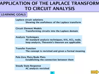
1. APPLICATION OF THE LAPLACE TRANSFORM TO CIRCUIT ANALYSIS LEARNING GOALS Laplace circuit solutions Showing the usefulness of the Laplace transform Circuit Element Models Transforming circuits into the Laplace domain Analysis Techniques All standard analysis techniques, KVL, KCL, node, loop analysis, Thevenin’s theorem are applicable Transfer Function The concept is revisited and given a formal meaning Pole-Zero Plots/Bode Plots Establishing the connection between them Steady State Response AC analysis revisited

2. Comple mentary LAPLACE CIRCUIT SOLUTIONS We compare a conventional approach to solve differential equations with a technique using the Laplace transform “Take Laplace transform” of the equation Initial conditions are automatically included P a r t i c u l a r Only algebra is needed No need to search for particular or comple- mentary solutions

3. In the Laplace domain the differential equation is now an algebraic equation LEARNING BY DOING Use partial fractions to determine inverse Initial condition given in implicit form

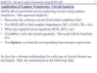
4. CIRCUIT ELEMENT MODELS Resistor The method used so far follows the steps: 1. Write the differential equation model 2. Use Laplace transform to convert the model to an algebraic form For a more efficient approach: 1. Develop s-domain models for circuit elements 2. Draw the “Laplace equivalent circuit” keeping the interconnections and replacing the elements by their s-domain models 3. Analyze the Laplace equivalent circuit. All usual circuit tools are applicable and all equations are algebraic.

5. Source transformation Impedance in series with voltage source Capacitor: Model 2 Impedance in parallel with current source Capacitor: Model 1

6. Inductor Models

7. Combine into a single source in the primary Single source in the secondary Mutual Inductance

8. Inductor with initial current Equivalent circuit in s-domain Determine the model in the s-domain and the expression for the voltage across the inductor LEARNING BY DOING Steady state for t<0

9. LEARNING EXAMPLE Draw the s-domain equivalent and find the voltage in both s-domain and time domain ANALYSIS TECHNIQUES All the analysis techniques are applicable in the s-domain One needs to determine the initial voltage across the capacitor

10. Do not increase number of loops Write the loop equations in the s-domain LEARNING EXAMPLE

11. Do not increase number of nodes Write the node equations in the s-domain LEARNING EXAMPLE

12. Node Analysis LEARNING EXAMPLE Assume all initial conditions are zero Could have used voltage divider here

13. Loop Analysis

14. Applying current source Current divider Applying voltage source Source Superposition Voltage divider

15. Combine the sources and use current divider Source Transformation The resistance is redundant

16. Reduce this part Using Thevenin’s Theorem Voltage divider Only independent sources

17. Reduce this part Using Norton’s Theorem Current division

18. LEARNING EXAMPLE Selecting the analysis technique: . Three loops, three non-reference nodes . One voltage source between non-reference nodes - supernode . One current source. One loop current known or supermesh . If v_2 is known, v_o can be obtained with a voltage divider Transforming the circuit to s-domain

19. Continued ... -keep dependent source and controlling variable in the same sub-circuit -Make sub-circuit to be reduced as simple as possible -Try to leave a simple voltage divider after reduction to Thevenin equivalent

20. Continued … Computing the inverse Laplace transform Analysis in the s-domain has established that the Laplace transform of the output voltage is One can also use quadratic factors...

21. supernode LEARNING EXTENSION Assume zero initial conditions Implicit circuit transformation to s-domain KCL at supernode

22. supermesh LEARNING EXTENSION Solve for I2 Determine inverse transform

23. LEARNING EXAMPLE Assume steady state for t<0 and determine voltage across capacitors and currents through inductors Circuit for t>0 TRANSIENT CIRCUIT ANALYSIS USING LAPLACE TRANSFORM For the study of transients, especially transients due to switching, it is important to determine initial conditions. For this determination, one relies on the properties: 1. Voltage across capacitors cannot change discontinuously 2. Current through inductors cannot change discontinuously

24. Laplace Use mesh analysis Solve for I2 Circuit for t>0 Now determine the inverse transform

25. Current divider LEARNING EXTENSION Initial current through inductor

26. LEARNING EXTENSION Determine initial current through inductor Use source superposition

27. System with all initial conditions set to zero TRANSFER FUNCTION H(s) can also be interpreted as the Laplace transform of the output when the input is an impulse and all initial conditions are zero The inverse transform of H(s) is also called the impulse response of the system If the impulse response is known then one can determine the response of the system to ANY other input

28. LEARNING EXAMPLE In the Laplace domain, Y(s)=H(s)X(s)

29. Normalized second order system Impulse response of first and second order systems First order system

30. Mesh analysis LEARNING EXAMPLE Transform the circuit to the Laplace domain. All initial conditions set to zero

31. Determine the transfer function, the type of damping and the unit step response LEARNING EXAMPLE Transform the circuit to the Laplace domain. All initial conditions set to zero

32. x O x Determine the pole-zero plot, the type of damping and the unit step response LEARNING EXTENSION

33. LEARNING EXAMPLE Normalized second order system Second order networks: variation of poles with damping ratio

34. The Tacoma Narrows Bridge Revisited LEARNING EXAMPLE Previously the event was modeled as a resonance problem. More detailed studies show that a model with a wind-dependent damping ratio provides a better explanation Torsional Resonance Model Problem: Develop a circuit that models this event

35. integrator adder model Using numerical values Simulation building blocks Simulation using dependent sources

36. Wind speed=20mph initial torsion=1 degree Wind speed=35mph initial torsion =1degree Simulation results

37. Bode plots display magnitude and phase information of Cross section shown by Bode POLE-ZERO PLOT/BODE PLOT CONNECTION They show a cross section of G(s) If the poles get closer to imaginary axis the peaks and valleys are more pronounced

38. Due to symmetry show only positive frequencies Front view Amplitude Bode plot Uses log scales Cross section

39. Response when all initial conditions are zero EXAMPLE transient Steady state response For the general case STEADY STATE RESPONSE Laplace uses positive time functions. Even for sinusoids the response contains transitory terms If interested in the steady state response only, then don’t determine residues associated with transient terms

40. Determine the steady state response LEARNING EXAMPLE Transform the circuit to the Laplace domain. Assume all initial conditions are zero

41. Thevenin LEARNING EXTENSION Transform circuit to Laplace domain. Assume all initial conditions are zero

42. De-emphasize bass Pole-zero map for Enhances bass to original level The playback filter is the reciprocal Pole/zero of playback filter cancels pole/zero of recording filter LEARNING BY APPLICATION

43. Proposed filter Design equations Well below 100k above 1k Filter design criteria Below 100k Filtering noise in a data transmission line LEARNING BY DESIGN Noise source is 100kHz Data bits at 1000bps SOLUTION: Insert a second order low-pass filter in the path. Should not affect data signal and should attenuate noise

44. Selected pole location or filter The filter eliminates noise but smooths data pulse 25kbps data transfer rate noise Filtered signal is useless Circuit simulating the filter REDESIGN!

45. New pole-zero selection Simulation for 25kbps APPLICATION LAPLACE