Download
1 / 10
100 likes | 133 Views
Learn about significance levels, errors in hypothesis testing, and the importance of discerning between statistical significance and practical significance. Dive into methods for selecting tests and interpreting results effectively in inferential statistics.

E N D
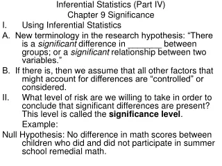
Inferential Statistics (Part IV) Chapter 9 Significance • Using Inferential Statistics A. New terminology in the research hypothesis: “There is a significant difference in _______ between groups; or a significant relationship between two variables.” B. If there is, then we assume that all other factors that might account for differences are “controlled” or considered. • What level of risk are we willing to take in order to conclude that significant differences are present? This level is called the significance level. Example: Null Hypothesis: No difference in math scores between children who did and did not participate in summer school remedial math.
Purpose of Research: Show that observed differences are due ONLY to the program and not other factors. By concluding that the differences in test scores are due to differences in program exposure, we accept some risk. The level of risk accepted (risk of being wrong by rejecting null) is the significance level. Say our significance level is .05. We are saying that there is only 1 chance in 20 (or 5 in 100) that any differences found were not due to the hypothesized reason (program) but to some other factor.
Errors (Type I and Type II) A. Type I error: the null is true and you reject it. The significance level refers to how much risk we are willing to accept. If we set it at .05, then we are saying that there is a 5% chance that we are making a Type I error. The greater the standard the greater the chance. Easily controlled, just change the risk level. B. Type II: The null is false and you accept it. More subjects/cases, the closer to the true population, the lower the risk of making Type II errors. Not easily controlled, change the sample size.
Significance verses meaningfulness Just because a factor is significant, does not mean that it is meaningful. Sometimes, significant differences are negligible even if significant. Significance does not tell us how big the impact is, it only tells us if there is an impact. The more significant DOES NOT mean the larger the impact or strength. Example: Are you willing to retain children in Grade 1 if the retention program significantly raises their standardized test scores by one-half point?
Selecting a test (p. 166 Figure 9.1; Fall in Love With this Diagram) The test you select depends upon the data that you have and the question you are asking. • Steps of Significance Testing: • State the null: (ex: no difference between average number of men and women voting) • Set the significance level (.05): There is only a 5% chance that observed differences are due to chance (95% due to something else, like gender). • Select appropriate test statistic (figure 9.1): difference in means (next few chapters) • Compute test statistic or obtained value (use SPSS and formulas). • Determination of value needed for rejection of null using the appropriate table of critical values (corresponds to a significance level, usually 5%)
Compare obtained value to critical value • If obtained value is more extreme than critical (less than 5% of all values), reject null. If not, do not reject null (chance is most reasonable explanation). That is: if ov>cv, reject null. If ov<cv, do not reject null. See Fig 9.2.
Chapter 10T-test for independent means Why? When you want to know if there are significant differences in characteristics (average income) between two independent groups (south/nonsouth).
Example: page 164 Steps: 1. Null: No difference between Group 1 and 2 Research: Difference between Group 1 and 2. • Set significance level: .05 • Select Appropriate test statistic: t-test independent samples (differences between different groups) • Compute test statistic (solve for t; do it by hand this time) • Determine value needed for rejection of null (find appropriate critical value in Table B2, Appendix B, p. 333)
determine degrees of freedom (df for this test-stat is n1- 1 + n2-1 or the sum of both groups (30+30=60) – 2, which is 58. • Find your df (58) and the appropriate significance level (.05) • The one tailed test is appropriate ONLY if the direction of the relationship is hypothesized (a directional-hypo; easier to pass a one-tailed test). 6. Compare critical (from table) and obtained value Obtained = -.14 and critical value is 2.001. Reject the null? • Do not reject null because the obtained value (-.14) does not exceed the critical value (2.001). Differences are probably due to random chance.
Using SPSS to conduct t-tests of independent samples • Get Troy’s state data • Analyze, compare means, independent-samples t-test • Click on income (adjincom) for test variable • Move grouping variable over to grouping variable box • Click define groups (and insert appropriate values) • Click okay or ok Another example: same thing comparing GOP controlled state gov’ts and others on % college educated.