Download
1 / 60
610 likes | 876 Views
7- Speech Recognition. Speech Recognition Concepts Speech Recognition Approaches Recognition Theories Bayse Rule Simple Language Model P(A|W) Network Types. 7- Speech Recognition (Cont’d). HMM Calculating Approaches Neural Components Three Basic HMM Problems Viterbi Algorithm

E N D
7-Speech Recognition • Speech Recognition Concepts • Speech Recognition Approaches • Recognition Theories • Bayse Rule • Simple Language Model • P(A|W) Network Types
7-Speech Recognition (Cont’d) • HMM Calculating Approaches • Neural Components • Three Basic HMM Problems • Viterbi Algorithm • State Duration Modeling • Training In HMM
Recognition Tasks • Isolated Word Recognition (IWR) Connected Word (CW) , And Continuous Speech Recognition (CSR) • Speaker Dependent, Multiple Speaker, And Speaker Independent • Vocabulary Size • Small <20 • Medium >100 , <1000 • Large >1000, <10000 • Very Large >10000
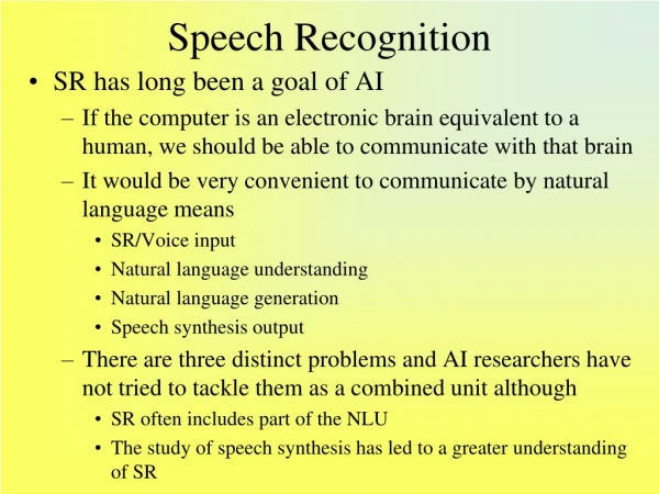
Speech Recognition Concepts Speech recognition is inverse of Speech Synthesis Speech Text NLP Speech Processing Speech Synthesis Understanding NLP Speech Processing Speech Phone Sequence Text Speech Recognition
Speech Recognition Approaches • Bottom-Up Approach • Top-Down Approach • Blackboard Approach
Bottom-Up Approach Signal Processing Voiced/Unvoiced/Silence Feature Extraction Segmentation Sound Classification Rules Signal Processing Knowledge Sources Phonotactic Rules Feature Extraction Lexical Access Segmentation Language Model Segmentation Recognized Utterance
Top-Down Approach Inventory of speech recognition units Word Dictionary Task Model Grammar Semantic Hypo thesis Syntactic Hypo thesis Unit Matching System Lexical Hypo thesis Feature Analysis Utterance Verifier/ Matcher Recognized Utterance
Blackboard Approach Acoustic Processes Lexical Processes Black board Environmental Processes Semantic Processes Syntactic Processes
Recognition Theories • Articulatory Based Recognition • Use from Articulatory system for recognition • This theory is the most successful until now • Auditory Based Recognition • Use from Auditorysystem for recognition • Hybrid Based Recognition • Is a hybrid from the above theories • Motor Theory • Model the intended gesture of speaker
Recognition Problem • We have the sequence of acoustic symbols and we want to find the words that expressed by speaker • Solution : Finding the most probable of word sequence by having Acoustic symbols
Recognition Problem • A : Acoustic Symbols • W : Word Sequence • we should find so that
Simple Language Model Computing this probability is very difficult and we need a very big database. So we use from Trigram and Bigram models.
Simple Language Model (Cont’d) Trigram : Bigram : Monogram :
Simple Language Model (Cont’d) Computing Method : Number of happening W3 after W1W2 Total number of happening W1W2 AdHoc Method :
Error Production Factor • Prosody (Recognition should be Prosody Independent) • Noise (Noise should be prevented) • Spontaneous Speech
P(A|W) Computing Approaches • Dynamic Time Warping (DTW) • Hidden Markov Model (HMM) • Artificial Neural Network (ANN) • Hybrid Systems
Dynamic Time Warping Method (DTW) • To obtain a global distance between two speech patterns a time alignment must be performed Ex : A time alignment path between a template pattern “SPEECH” and a noisy input “SsPEEhH”
Artificial Neural Network . . . Simple Computation Element of a Neural Network
Artificial Neural Network (Cont’d) • Neural Network Types • Perceptron • Time Delay • Time Delay Neural Network Computational Element (TDNN)
Artificial Neural Network (Cont’d) Single Layer Perceptron . . . . . .
Artificial Neural Network (Cont’d) Three Layer Perceptron . . . . . . . . . . . .
Hybrid Methods • Hybrid Neural Network and Matched Filter For Recognition Acoustic Features Output Units Speech Delays PATTERN CLASSIFIER
Neural Network Properties • The system is simple, But too much iteration is needed for training • Doesn’t determine a specific structure • Regardless of simplicity, the results are good • Training size is large, so training should be offline • Accuracy is relatively good
Hidden Markov Model • Observation : O1,O2, . . . • States in time : q1, q2, . . . • All states : s1, s2, . . ., sN Sj Si
Hidden Markov Model (Cont’d) • Discrete Markov Model Degree 1 Markov Model
Hidden Markov Model (Cont’d) : Transition Probability from Si to Sj ,
Discrete Markov Model Example S1 : The weather is rainy S2 : The weather is cloudy S3 : The weather is sunny cloudy sunny rainy rainy cloudy sunny
Hidden Markov Model Example (Cont’d) Question 1:How much is this probability: Sunny-Sunny-Sunny-Rainy-Rainy-Sunny-Cloudy-Cloudy
Hidden Markov Model Example (Cont’d) The probability of being in state i in time t=1 Question 2:The probability of staying in state Si for d days if we are in state Si? d Days
Discrete Density HMM Components • N : Number Of States • M : Number Of Outputs • A (NxN) : State Transition Probability Matrix • B (NxM): Output Occurrence Probability in each state • (1xN): Initial State Probability : Set of HMM Parameters
Three Basic HMM Problems • Given an HMM and a sequence of observations O,what is the probability ? • Given a model and a sequence of observations O, what is the most likely state sequence in the model that produced the observations? • Given a model and a sequence of observations O, how should we adjust model parameters in order to maximize ?
First Problem Solution We Know That: And
First Problem Solution (Cont’d) Computation Order :
Forward Backward Approach Computing 1) Initialization
Forward Backward Approach (Cont’d) 2) Induction : 3) Termination : Computation Order :
Backward Variable 1) Initialization 2)Induction
Second Problem Solution • Finding the most likely state sequence Individually most likely state :
Viterbi Algorithm • Define : P is the most likely state sequence with this conditions : state i , time t and observation o
Viterbi Algorithm (Cont’d) 1) Initialization Is the most likely state before state i at time t-1
Viterbi Algorithm (Cont’d) 2) Recursion
Viterbi Algorithm (Cont’d) 3) Termination: 4)Backtracking:
Third Problem Solution • Parameters Estimation using Baum-Welch Or Expectation Maximization (EM) Approach Define:
Third Problem Solution (Cont’d) : Expectation value of the number of jumps from state i : Expectation value of the number of jumps from state i to state j
Baum Auxiliary Function By this approach we will reach to a local optimum
Continuous Observation Density • We have amounts of a PDF instead of • We have Mixture Coefficients Variance Average
Continuous Observation Density • Mixture in HMM M1|1 M1|2 M1|3 M2|1 M2|2 M2|3 M3|1 M3|2 M3|3 M4|1 M4|2 M4|3 S2 S3 S1 Dominant Mixture: